XLSX Templates

Introduction

This section will go through all the tags that are available for the XLSX template, together with the appropriate data selection query. In this documentation, curly braces {...} are used as delimiters for the tags. Please check the general template for how to change the delimiters delimiters. The templates can be made using various software like Microsoft Excel, LibreOffice Calc, APEX Office Edit, or Google Sheets. The files should be in .xlsx or .xlsm format.

Tag Overview

The following tables show the available tags in the XLSX template. The three dots in the format column shows what is variable, they should be either replaced by the cursor name or column name.

info

Please note that the column names are case-sensitive, you can use double quotes to force the casing.

Tags can't start with a number and should start with an alphabetical character (a-z, A-Z)

Tag Name	Format	Tag Example	Short Description
Normal Substitution	{...}	{normal}	Normal Substitution, the data from the given column will be replaced.
Normal Substitution with cell markup	{...$}	{normal_with_cell_markup$}	Normal Substitution with various styling options The data from the given column will be replaced along with the styling.
Html Content	{_...}	{_htmlContent}	Tag to be used when the content of a column is HTML content.
Sheet Generation	{!...}	{!sheet_loop}	Tag to be used when generating individual sheets for each record, where each sheet have information of a record.
Loop Tags	{#...} {/...}	{#data_loop} … {/data_loop}	Tag that loops over the given cursor name and repeats everything in between the tags for each record by creating new row(s).
Horizontal Loop Tags	{:...} {/...}	{:data_loop_horizontal} … {/data_loop_horizontal}	Tag to be used when repeating columns. Will repeat the given column(s) for the given cursor.
Table row Loop	{=...} {/...}	{=table_row_loop} … {/table_row_loop}	Tag to be used when merging cells of column.
Image	{%...}	{%imageKey}	Tag to be used when the content is an image. (can point to URL, file, base64encoded string) Options available see details
Barcode and QR Code	{|...}	{|barcode_or_qrcode}	Tag to use when a barcode or QR code needs to be generated in its place. Options available see details.
QR Code Image Replacing	QR code of Tag	QR code of Tag	Tag to be used when the content is an image, barcode, or QR code but needs custom styling. Options available see details
Chart	{$...}	{$chart}	Tag to be used when a native Excel chart should be generated, see details for the specific format of what this cursor should contain.
AOP Chart	{aopchart ...}	{aopchart chartData}	Tag to be used near a chart that is defined and styled in the template, see details for passing the data for this dummy chart.
D3 Images	{$d3 ...}	{$d3 image_data}	Tag to be used to insert d3 images on Excel sheet.
Interactive Report	{&interactive}	{&interactive} or {&interactive_1}	Tag to be used when the data source is an interactive report. This will recreate the given interactive report in Excel.
Interactive Grid	{&...&}	{&interactive_grid&}	Tag to be used as the data source is an interactive grid.
Classic Report	{&...&}	{&classic_report&}	Tag to be used for the data source is a classic report.
Hyperlink	{*...}	{*hyperlink}	Substitution like normal tag, but will contain a hyperlink so that a user can be directed.
Auto Link	{*auto ...}	{*auto text}	Substitution like normal tag, but will detect if there are any hyperlinks, if so then a hyperlink will be created.
Span	{...#}	{span#}	Tag to be used when creating the span of a cell to row(s) and column(s).
Static Condition	{##...}	{##static_condition}	Tag to be used to create a conditional block where rows will not be pushed back when the condition fails.
Formula	{>...}	{>formula}	Tag to be used when inserting Excel formula in a cell.
Page Break	{?...}	{?pageBreak}	Tag that will insert a page break when the provided condition evaluates to true.
Text Box	{tbox ...}	{tbox text}	Tag will create a text box at a given position. Options are available to see details.
Freeze Pane	{freeze ...}	{freeze freezePane}	Tag to be used to freeze cell(s)/pane. Options available see details.
Sheet Protection	{protect ...}	{protect tagName}	Tag to be used to protect a cell. Options available see details.
Insert Document	{?insert ...}	{?insert insertDocument}	Tag that will attach the given document(docx, ppt, XLSX, PDF) inside the template/output. Options available see details.
Skip	{skip}	{skip}	Tag to be used to skip the rendering of the Excel sheet. Used with sheet name.
Hide Sheets	{hide ...}	{hide condition}	Tag to be used to hide sheet(s) in workbook for a given condition.
Delete Sheets	{delete ...}	{delete condition}	Tag to be used to delete sheet(s) in workbook for a given condition.
Hide Columns	{hideColumn ...}	{hideColumn condition}	Tag to be used to hide column(s) in workbook for a given condition.
Hide Rows	{hideRow ...}	{hideRow condition}	Tag to be used to hide row(s) in workbook for a given condition.
Cell Validation	{validate ...}	{validate validateTag}	Tag to be used to insert cell validation in a cell of Excel sheet.

tip

Special Tags: Other special tags can be used. Please refer to the general template section: special-tags

Normal Substitution

Available From: v1.0

These kinds of tags are the simplest tag to use. These tags are enclosed in curly braces and can include variables (name of the column) that will be replaced with actual data when the output is generated. The replaced value will have the same style as the tag itself. To be more specific the style of starting curly brace. This info might be useful when the tag is long. In this case, you can style the starting curly braces and change the font of the remaining tag to a smaller size.

eg: {cust_first_name}. This font size of output text would be the size of the first curly brace.

Tag with different style

In Excel, multiple tags with different styling can be assigned to a single cell, and these styles will be preserved when processed using AOP.
For instance, suppose the template contains a cell with {text1} {text2}, and your data source is:

'Hello this is first text' as "text1",
'This is second text' as "text2"

If above are processed with AOP, Hello this is first text This is second text is produced.

Example

The data source below was created using the database available in the sample data of AOP. The database contains numerous tables and views with raw data that can be used for reference.

Date Source

Hereby example data source for different options.

SQL

select
  'file1' as "filename",
  cursor (
    select
      c.cust_first_name as "cust_first_name",
      c.cust_last_name as "cust_last_name"
    from
      aop_sample_customers c
    where
      c.customer_id = 1
  ) as "data"
from
  dual

PL/SQL returning SQL

declare l_return clob;

begin l_return := q '[
        select
            ' file1 ' as "filename",
            cursor (
                select
                    c.cust_first_name as "cust_first_name",
                    c.cust_last_name as "cust_last_name"
                    from aop_sample_customers c
                    where c.customer_id = 1
            ) as "data"
        from dual
        ]';

return l_return;

end;

PL/SQL returning JSON

declare l_cursor sys_refcursor;
l_return clob;
begin apex_json.initialize_clob_output(dbms_lob.call, true, 2);
open l_cursor for
select
  'file1' as "filename",
  cursor (
    select
      c.cust_first_name as "cust_first_name",
      c.cust_last_name as "cust_last_name"
    from
      aop_sample_customers c
    where
      c.customer_id = 1
  ) as "data"
from
  dual;
apex_json.write(l_cursor);
l_return := apex_json.get_clob_output;

/*
 l_return can also be a varchar2:
 l_return := q'[
  [
    {
    "filename": "file1",
    "data": [
          {
          "cust_first_name": "John",
          "cust_last_name": "Dulles"
          }
      ]
    }
  ]
 ]';
 */
return l_return;

end;

JSON

[
  {
    "filename": "file1",
    "data": [
      {
        "cust_first_name": "John",
        "cust_last_name": "Dulles"
      }
    ]
  }
]

Template

The template should contain the name of the columns that were provided in the query above. For example, we have the template with the following content:

Hello {cust_first_name} {cust_last_name},

This is the basic example of using normal tags.
Thank you for choosing AOP.

Best Regards,
AOP Team

 template.xlsx  

Output

When the above data source (which results in one row with John as cust_first_name and Dulles as cust_last_name) and the given template are passed to AOP, the output will be as follows.

Hello John Dulles,

This is the basic example of using normal tags.
Thank you for choosing AOP.

Best Regards,
AOP Team

 output.xlsx  

Cell Markup

Available From: v3.0

AOP enables users to format Excel text and cells using cell markup tags that consist of a column name followed by a dollar sign enclosed in delimiters. These tags support various styling options, including font, font size, font style, background color, height, and width, among others. The available formatting options include:

• cell_locked : [y/n]
• cell_hidden : [y/n]
• cell_background : hex color e.g: #ff0000
• font_name : name of the font e.g: Arial
• font_size : e.g 14, Note: no unit is considered px. For fonts with 14 points use ("14pt"). Supported units: inch, cm, px, pt, em, Excel Units(eu).
• font_color : hex color e.g: #00ff00
• font_italic : [y/n]
• font_bold : [y/n]
• font_strike : [y/n]
• font_underline : [y/n]
• font_superscript :[y/n]
• font_subscript :[y/n]
• border_top : [dashed / dashDot / hair / dashDotDot / dotted / mediumDashDot / mediumDashed / mediumDashDotDot / slantDashDot / medium / double / thick ]
• border_top_color : hex color e.g: #000000
• border_bottom : [dashed / dashDot / hair / dashDotDot / dotted / mediumDashDot / mediumDashed / mediumDashDotDot / slantDashDot / medium / double / thick ]
• border_bottom_color : hex color e.g: #000000
• border_left : [dashed / dashDot / hair / dashDotDot / dotted / mediumDashDot / mediumDashed / mediumDashDotDot / slantDashDot / medium / double / thick ]
• border_left_color : hex color e.g: #000000
• border_right : [dashed / dashDot / hair / dashDotDot / dotted / mediumDashDot / mediumDashed / mediumDashDotDot / slantDashDot / medium / double / thick ]
• border_right_color : hex color e.g: #000000
• border_diagonal : [dashed / dashDot / hair / dashDotDot / dotted / mediumDashDot / mediumDashed / mediumDashDotDot / slantDashDot / medium / double / thick ]
• border_diagonal_direction : [up-wards|down-wards| both]
• border_diagonal_color : hex color e.g: #000000
• text_h_alignment : [top|bottom|center|justify]
• text_v_alignment : [top|bottom|center|justify]
• text_rotation : rotation of text value from 0-90 degrees
• wrap_text : set it true for wrap text. The default is false.
• width : We can provide a custom width to the cell. Supported units: inch, cm, px, pt, em, Excel Units(eu) Note: If the column is created using horizontal looping, then only the width can be decreased, however, the width can be increased always and max width of all cells of a column is considered as column width.
• height : We can provide custom height to the cell. Supported units: inch, cm, px, pt, em, Excel Units(eu) Note: If the column is created using vertical looping, then only the height can be decreased, however, height can be increased always and max height of all cells of the row is considered as row height.
• max_characters : This can also be used to provide width for the cell. Use height as an auto to see the magic.
• height_scaling: When the cell height may not be as expected. For some fonts and styling AOP may not be able to calculate the height of the cell accurately. In this case, you can provide the height_scaling, in terms of percentage or number(considering 1 is 100%). If the height is smaller than expected, you can set this attribute to 1.3 or "130%" according to your requirement. Note: Office Excel and LibreOffice Calc renders the same document differently, so, if your output is pdf (using default or libreoffice as converter), you can set this attribute to 0.75 or (75%) thus creating expected height of cell. Available from 22.2.5

For ex: If you want to change the font_color of the text. Let's say your column name is text. Set the value for text_font_color as color name or hex value.

'Hello!' as "text",
'DeepSkyBlue' as "text_font_color"

the tag {text$} outputs Hello! in DeepSkyBlue.

Since AOP version 19.2 it is possible to give the number format with the styles:

• format_mask : "999G999G999G999G990D00PR"
• currency : "$"

Since AOP 19.3, the same format_mask option can also be specified as a date format mask, e.g. "MM/DD/YYYY", for data which matches an ISO 8601 date.

Together with the format mask, we've added the possibility to adjust the height and width of the cells. We expect the following data:

• width : "auto" or number (in pixels) (optional)
• height : "auto" or number (in pixels) (optional)
• wrap_text : true or false
• max_characters : Number //max character per line

Please note that if the tag is {example$} is used, then the data provided should be inside example_cell_background, example_font_italic, etc. If you are using the format mask, then the Excel settings will define which thousand separator and decimal separator to use.

Since version 19.2.1 you can also provide a custom Excel format, i.e. the format mask provided will be placed into the Excel cell without modifications. The format mask should start with "excel:" followed by the format mask. e.g.:

excel:#,##0.00;[Red]-#,##0.00
Usage:

'2500' as "example",
'excel:#,##0.00;[Red]-#,##0.00' as "example_format_mask"

Note: To use the options provided above, you should join the tag name and option name using an underscore character (\_).

Excel Units

Available From: v22.2.4

From AOP version 22.2.4, It is possible to provide Excel Units(EU) as the unit of measurement.

In the above image, the width of the column is 14.29 Excel Units or 105 pixels. This column of the worksheet will have the same Excel Units, but pixels can vary according to the display resolution. It is recommended to provide Excel Units(EU), Ex (15eu) for precise measurement while providing the width of the cell.

Example

The data source below was created using the database available in the sample data of AOP. The database contains numerous tables and views with raw data that can be used for reference.

Data Source

Hereby are examples of data sources for different options.

SQL

select
  'file1' as "filename",
  cursor(
    select
      c.cust_first_name as "cust_first_name",
      c.cust_last_name as "cust_last_name",
      -- for styling
      'Hello from AOP' as "text",
      'Arial' as "text_font_name",
      'y' as "text_font_italic",
      'n' as "text_font_strike",
      'dashed' as "text_border_top",
      'red' as "text_font_color",
      -- for width and height
      'Hello this is long text and might need to set different width.' as "text2",
      '40' as "text2_width",
      '30pt' as "text2_height",
      'true' as "text2_wrap_text",
      -- for format max
      '25000' as "text3",
      '999G999G999G999G990D00PR' as "text3_format_mask",
      '$' as "text3_currency",
      -- for max_characters
      'Fictum, deserunt mollit anim laborum astutumque! Quisque placerat facilisis egestas cillum dolore. Nec dubitamus multa iter quae et nos invenerat. Contra legem facit qui id facit quod lex prohibet. Quam diu etiam furor iste tuus nos eludet?' as "text4",
      30 as "text4_max_characters",
      'true' as "text4_wrap_text",
      'auto' as "text4_height"
    from
      aop_sample_customers c
    where
      c.customer_id = 1
  ) as "data"
from
  dual

PL/SQL returning SQL

declare l_return clob;

begin l_return := q '[
        select
          'file1' as "filename",
          cursor(
            select
              c.cust_first_name as "cust_first_name",
              c.cust_last_name as "cust_last_name",
              -- for styling
              'Hello from AOP' as "text",
              'Arial' as "text_font_name",
              'y' as "text_font_italic",
              'n' as "text_font_strike",
              'dashed' as "text_border_top",
              'red' as "text_font_color",
              -- for width and height
              'Hello this is long text and might need to set different width.' as "text2",
              '40' as "text2_width",
              '30pt' as "text2_height",
              'true' as "text2_wrap_text",
              -- for format max
              '25000' as "text3",
              '999G999G999G999G990D00PR' as "text3_format_mask",
              '$' as "text3_currency",
              -- for max_characters
              'Fictum, deserunt mollit anim laborum astutumque! Quisque placerat facilisis egestas cillum dolore. Nec dubitamus multa iter quae et nos invenerat. Contra legem facit qui id facit quod lex prohibet. Quam diu etiam furor iste tuus nos eludet?' as "text4",
              30 as "text4_max_characters",
              'true' as "text4_wrap_text",
              'auto' as "text4_height"
            from
              aop_sample_customers c
            where
              c.customer_id = 1
          ) as "data"
        from
          dual
        ]';
return l_return;

end;

PL/SQL returning JSON

declare l_cursor sys_refcursor;

l_return clob;

begin apex_json.initialize_clob_output(dbms_lob.call, true, 2);

open l_cursor for
select
  'file1' as "filename",
  cursor(
    select
      c.cust_first_name as "cust_first_name",
      c.cust_last_name as "cust_last_name",
      -- for styling
      'Hello from AOP' as "text",
      'Arial' as "text_font_name",
      'y' as "text_font_italic",
      'n' as "text_font_strike",
      'dashed' as "text_border_top",
      'red' as "text_font_color",
      -- for width and height
      'Hello this is long text and might need to set different width.' as "text2",
      '40' as "text2_width",
      '30pt' as "text2_height",
      'true' as "text2_wrap_text",
      -- for format max
      '25000' as "text3",
      '999G999G999G999G990D00PR' as "text3_format_mask",
      '$' as "text3_currency",
      -- for max_characters
      'Fictum, deserunt mollit anim laborum astutumque! Quisque placerat facilisis egestas cillum dolore. Nec dubitamus multa iter quae et nos invenerat. Contra legem facit qui id facit quod lex prohibet. Quam diu etiam furor iste tuus nos eludet?' as "text4",
      30 as "text4_max_characters",
      'true' as "text4_wrap_text",
      'auto' as "text4_height"
    from
      aop_sample_customers c
    where
      c.customer_id = 1
  ) as "data"
from
  dual
apex_json.write(l_cursor);

l_return := apex_json.get_clob_output;

return l_return;

end;

JSON

[
  {
    "filename": "file1",
    "data": [
      {
        "cust_first_name": "John",
        "cust_last_name": "Doe",
        "text": "Hello from AOP",
        "text_font_name": "Arial",
        "text_font_italic": "y",
        "text_font_strike": "n",
        "text_border_top": "dashed",
        "text_font_color": "red",
        "text2": "Hello this is long text and might need to set different width.",
        "text2_width": 40,
        "text2_height": "30pt",
        "text2_wrap_text": true,
        "text3": 25000,
        "text3_format_mask": "999G999G999G999G990D00PR",
        "text3_currency": "$",
        "text4": "Fictum, deserunt mollit anim laborum astutumque! Quisque placerat facilisis egestas cillum dolore. Nec dubitamus multa iter quae et nos invenerat. Contra legem facit qui id facit quod lex prohibet. Quam diu etiam furor iste tuus nos eludet?",
        "text4_max_characters": 30,
        "text4_wrap_text": true,
        "text4_height": "auto"
      }
    ]
  }
]

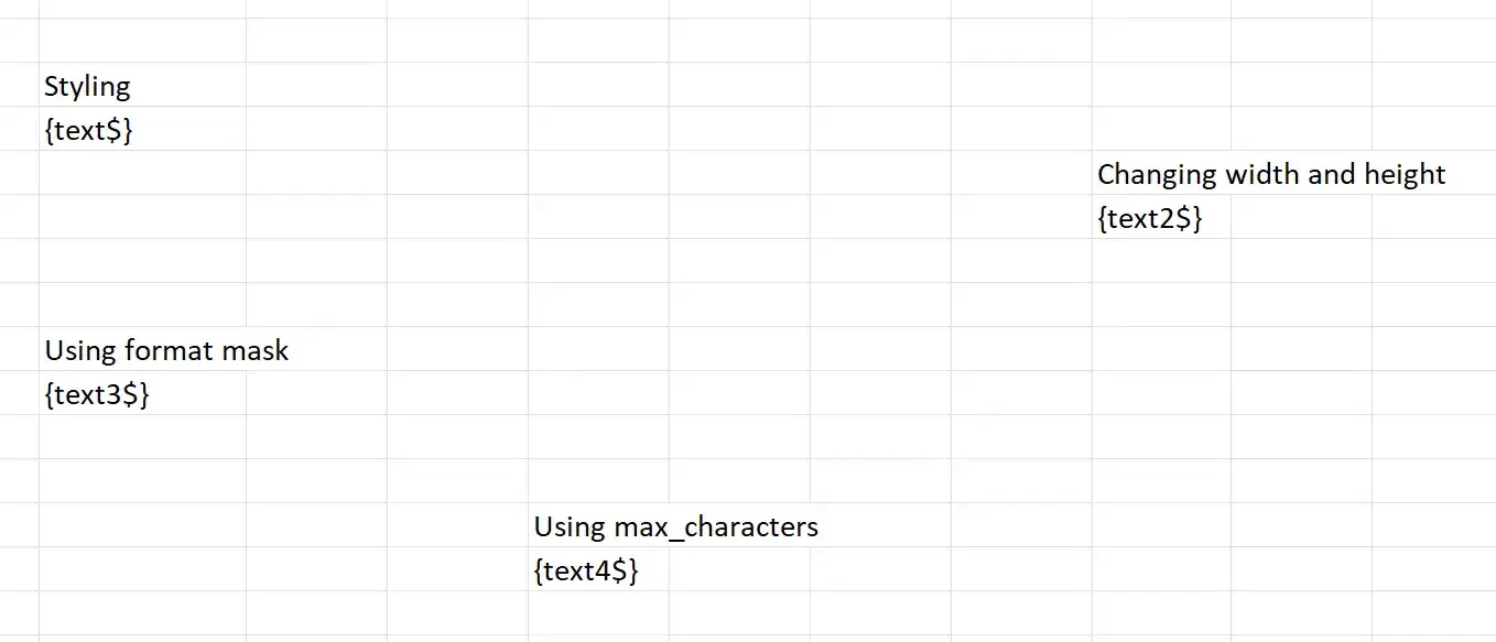
Template

The template should contain the cell markup tag which ends with a dollar sign ($). For example, we have the template with the following content:

 template.xlsx  

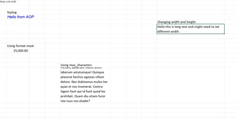
Output

When the above data source (which results in a row with columns as styling.) and the given template are passed to AOP, the output will be as follows.

 output.xlsx  

HTML Content

Available From: v2.1

Starting from AOP v2.1, HTML tags can now be inserted into Excel using the HTML tags (_ followed by column name enclosed within delimiters). This enables the conversion of HTML within Excel. The following subsections will provide more detailed explanations of the usage of tags and styling options. The tags and styling options that are presently supported are listed below.

Supported HTML Tags

Tag	Description
<br />	in order to introduce breaks (newline)
<p> .. </p>	represents a paragraph
<strong> .. </strong>	bold text
<b> .. </b>	bold text
<s> .. </s>	strike through
<u> .. </u>	underline
<em> .. </em>	italics
<h1> .. </h1>	heading 1
<h2> .. </h2>	heading 2
<h3> .. </h3>	heading 3
<h4> .. </h4>	heading 4
<h5> .. </h5>	heading 5
<h6> .. </h6>	heading 6
<sub> .. </sub>	subscript
<sup> .. </sup>	superscript
<ol> .. </ol>	ordered list
<ul> .. </ul>	unordered list
<li> .. </li>	list item
<table> .. </table>	table (including th, tr, td)
<caption> .. </caption>	caption
<img>	image
<pre> .. </pre>	preformatted text
<blockquote>.</blockquote>	quoting for multiple lines
<q> .. </q>	quoting for single line
<dfn> .. </dfn>	definition element
<span style="..">..</span>	text between the span will have the style defined, background-color, color, font-size and font-family are supported.

The following properties are inline CSS styling properties. Their general usage should be in the format of style="inlineCSSpropert : stylingParameter;". The syntax is important. After the inlineCSSproperty there must be a double dot and after the styling parameter there must be a semicolon. For example:
<p style="background-color: yellow;">

color               : Specifies the color of the text. (e.g.: red, #00ff00, rgb(0,0,255))
font-size           : Sets the size of a font. (e.g.: 15px, large)
font-style          : The font style for a text (e.g.: italic, oblique)
font-weight         : The font style for a text (e.g.: bold)
text-decoration     : The decoration added to the text (e.g.: underline, line-through)
background-color    : The background color of an element (e.g.: red, #00ff00, rgb(0,0,255))
text-indent         : The indentation of the first line in a text block (e.g.: 5px)
vertical-align      : The vertical alignment of an element (e.g.: baseline, text-top, text-bottom)
text-align          : The horizontal alignment of text in an element (e.g.: center, left, right)
border-style        : This property defines the appearance of the borders of an element and can take up to four values that correspond to the styles of the top, right, bottom, and left borders. For example, the border styles could be any combination of dotted, solid, double, and dashed.
border-color        : An element can have up to four border colors, with the possibility of having different values assigned to each border (e.g. red, green, blue, pink).
border-right        : Defines a border for the right part of the element. The border-right is a shorthand property for border-right-width, border-right-style (required), and border-right-color. (e.g.: 5px solid red)
                      However, the border-right-width property is not supported due to the limitations of Excel. One can still define width but it will be omitted. If two values will be defined they must only contain style and color information.
border-left         : Defines a border for the left part of the element. The same rules apply to border-right.
border-top          : Defines a border for the top part of the element. The same rules apply to border-right.
border-bottom       : Defines a border for the bottom part of the element. The same rules apply to border-right.
font-family         : Specifies the font for an element. (e.g.: Times New Roman (<span className='small-note'>note that it is provided without quotation mark</span>), Arial)

General Overview

While preparing an HTML code for AOP, we need to consider a few requirements regarding the HTML syntax and the limitations imposed by Excel. We will discuss those requirements lower. Now let's take a look at a sample usage of this new tag. In the below example, we provided an example that contains almost all of the tags that are supported.

<p>This is text coming from the database/session in HTML format.
    <br />It supports:
</p>
<ol>
    <li>Lists</li>
    <li><strong>Bold</strong></li>
    <li><em>Italic</em></li>
    <li><u>Underline</u></li>
    <li><s>Strikethrough</s></li>
    <li>Sub<sub>script</sub></li>
    <li><sup>Super</sup>script</li>
    <li><small>Small</small></li>
    <li style="color:#FF0000;">Text Color</li>
    <li style="background-color:#FFFF00;">Background Text Color</li>
</ol>

<h1>Heading 1</h1>
<h2>Heading 2</h2>
<h3>Heading 3</h3>
<h4>Heading 4</h4>
<h5>Heading 5</h5>
<h6>Heading 6</h6>

<table style="border-style: solid; border-color: red;">
    <tr>
        <th>Headers</th>
        <th>Borders</th>
    </tr>
    <tr>
        <td>Border Color</td>
        <td>Font Color</td>
    </tr>
</table>

This will result in the following Excel file:

Block and Inline Elements

When using HTML inside Excel, we are limited by the cell structure of Excel. Because of this reason using proper HTML syntax in terms of Block and Inline elements is crucial for getting correct results. Below, one can find all of the block and inline elements that AOP supports.

Block Elements	Inline Elements
\<div>	\<u>
\<h1> - \<h6>	\<b>
\<li>	\<br>
\<ol>	\<em>
\<p>	\<i>
\<table>	\<img>
\<ul>	\<small>
\<th>	\<span>
\<td>	\<strong>
\<a>	\<sub>
	\<sup>
	\<var>
	\<s>
	\<del>
	\<ins>

The block elements' scope can be considered as a single Excel cell and inline elements are the elements that are inside block elements.
Not all CSS styling elements are supported by Excel templates. The below table summarizes the supported CSS styling options.

Block Level Styling	Inline Level Styling
background-color	color
text-indent	font-size
vertical-align	font-style
text-align	font-weight
border-style	text-decoration
border-color	font-family
border-right
border-left
border-top
border-bottom

In this table, the most important part is block level styling elements. Inline-level styling can be used with any sort of HTML tags, but block-level styling elements can only be used with block-level elements.

<table> Tag

HTML tables are either placed in Excel tables or placed in the format of a table. If the table that wanted to be placed in Excel contains headers, or <th> elements, it will be rendered as an Excel table otherwise it will be placed in the form of a table.
Below is a table example with <th>,

<table>
    <tr>
        <th>Table Header 1</th>
        <th>Table Header 2</th>
    </tr>
    <tr>
        <td>Table Data 1</td>
        <td>Table Data 2</td>
    </tr>
</table>

It will look like the below picture.

Below is a table example just with <td>,

<table>
    <tr>
        <td>Table Header 1</td>
        <td>Table Header 2</td>
    </tr>
    <tr>
        <td>Table Data 1</td>
        <td>Table Data 2</td>
    </tr>
</table>

It will look like the below picture.

Currently, AOP doesn't support Block Level Elements inside tables.

<ol> and <ul> Tags

Ordered lists, <ol>, and unordered lists, <ul>, can be nested within each other and within any other element that is currently supported by AOP. Below is an example containing nested ordered lists and unordered lists.

<ol>
    <li>Ordered Level 1.1</li>
    <li>Ordered Level 1.2</li>
    <li>Ordered Level 1.3 <ol>
            <li>Ordered Level 2.1</li>
            <li>Ordered Level 2.2 <ol>
                    <li>Ordered Level 3.1</li>
                    <li>Ordered Level 3.2</li>
                    <li>Ordered Level 3.3</li>
                </ol>
            </li>
            <li>Ordered Level 2.3</li>
        </ol>
    </li>
    <li>Ordered Level 1.4
        <ul>
            <li>Unordered Level 1.1</li>
            <li>Unordered Level 1.2 
                <table>
                    <tr>
                        <td>Table Header 1</td>
                        <td>Table Header 2</td>
                        <td>Table Header 3</td>
                    </tr>
                    <tr>
                        <td>Table data 1</td>
                        <td>Table <b>data</b> 2</td>
                        <td>Table data 3</td>
                    </tr>
                    <tr>
                        <td>Tab<i>le<small><u>da</u></small>ta</i> 4</td>
                        <td>Table data 5</td>
                        <td>Table data 6</td>
                    </tr>
                    <tr>
                        <td>Table data 7</td>
                        <td>Table data 8</td>
                        <td>Table data 9</td>
                    </tr>
                </table>
            </li>
            <li>Unordered Level 1.3 <ul>
                    <li>Unordered <b>Level 2.1</b></li>
                    <li>Unordered <u>Level 2.2</u></li>
                    <li>Unordered Level 2.3 
                        <ul>
                            <li>Unordered Level 3.1</li>
                            <li>Unordered Level 3.2</li>
                            <li>Unordered Level 3.3</li>
                        </ul>
                    </li>
                </ul>
            </li>
        </ul>
    </li>
</ol>

The result will look like this,

For the ordered list starting value can be user-defined. This can be achieved through the start parameter in HTML. Given the below HTML code:

The result will look like below picture:

<ol start="10">
    <li>Item 1</li>
    <li>Item 2</li>
    <li>Item 3</li>
</ol>

<a> Tag

HTML hyperlinks, <a>, are supported by AOP. Below is an example of how to use it,

<a href="https://united-codes.com/index.html">United Code website</a>

This will result in the following way,

<img> Tag

HTML images, <img>, are supported by AOP. The source can be links, base64 encoded images, etc. Alt text, width, and height of the images can be optionally given. Below is an example of how to use it,

<img
  src="https://picsum.photos/seed/picsum/200/300"
  alt="Alt Text"
  width="500"
  height="500"
/>

This will result in the following picture,

Images can be used as hyperlinks as well. Below is an example of it,

<a href="https://united-codes.com/index.html"
  ><img
    src="https://picsum.photos/seed/picsum/200/300"
    alt="Alt Text"
    width="500"
    height="500"
/></a>

Example

The data source below was created using the database available in the sample data of AOP. The database contains numerous tables and views with raw data that can be used for reference.

Data Source

Hereby are examples of data sources for different options.

SQL

select
  'file1' as "filename",
  cursor (
    select
      c.cust_first_name as "cust_first_name",
      c.cust_last_name as "cust_last_name",
      '<p>This is text coming from the database / session in HTML format. <br />It supports: </p> <ol> <li>Lists</li> <li><strong>Bold</strong></li> <li><em>Italic</em></li> <li><u>Underline</u></li> <li><s>Strikethrough</s></li> <li>Sub<sub>script</sub></li> <li><sup>Super</sup>script</li> <li><small>Small</small></li> <li style=\"color:#FF0000;\">Text Color</li> <li style=\"background-color:#FFFF00;\">Background Text Color</li> </ol> <h1>Heading 1</h1> <h2>Heading 2</h2> <h3>Heading 3</h3> <h4>Heading 4</h4> <h5>Heading 5</h5> <h6>Heading 6</h6> <table style=\"border-style: solid; border-color: red;\"> <tr> <th>Headers</th> <th>Borders</th> </tr> <tr> <td>Border Color</td> <td>Font Color</td> </tr> </table>' as "htmlContent"
    from
      aop_sample_customers c
    where
      c.customer_id = 1
  ) as "data"
from
  dual

PL/SQL returning SQL

declare
    l_return clob;
begin
    l_return := q'[
        select
        'file1' as "filename",
        cursor (
          select
            c.cust_first_name as "cust_first_name",
            c.cust_last_name as "cust_last_name",
            '<p>This is text coming from the database / session in HTML format. <br />It supports: </p> <ol> <li>Lists</li> <li><strong>Bold</strong></li> <li><em>Italic</em></li> <li><u>Underline</u></li> <li><s>Strikethrough</s></li> <li>Sub<sub>script</sub></li> <li><sup>Super</sup>script</li> <li><small>Small</small></li> <li style=\"color:#FF0000;\">Text Color</li> <li style=\"background-color:#FFFF00;\">Background Text Color</li> </ol> <h1>Heading 1</h1> <h2>Heading 2</h2> <h3>Heading 3</h3> <h4>Heading 4</h4> <h5>Heading 5</h5> <h6>Heading 6</h6> <table style=\"border-style: solid; border-color: red;\"> <tr> <th>Headers</th> <th>Borders</th> </tr> <tr> <td>Border Color</td> <td>Font Color</td> </tr> </table>' as "htmlContent"
          from
            aop_sample_customers c
          where
            c.customer_id = 1
        ) as "data"
      from
        dual
        ]';
    return l_return;
end;

PL/SQL returning JSON

declare
  l_cursor sys_refcursor;
  l_return clob;
begin
  apex_json.initialize_clob_output(dbms_lob.call, true, 2) ;
  open l_cursor for
  select
    'file1' as "filename",
    cursor (
      select
        c.cust_first_name as "cust_first_name",
        c.cust_last_name as "cust_last_name",
        '<p>This is text coming from the database / session in HTML format. <br />It supports: </p> <ol> <li>Lists</li> <li><strong>Bold</strong></li> <li><em>Italic</em></li> <li><u>Underline</u></li> <li><s>Strikethrough</s></li> <li>Sub<sub>script</sub></li> <li><sup>Super</sup>script</li> <li><small>Small</small></li> <li style=\"color:#FF0000;\">Text Color</li> <li style=\"background-color:#FFFF00;\">Background Text Color</li> </ol> <h1>Heading 1</h1> <h2>Heading 2</h2> <h3>Heading 3</h3> <h4>Heading 4</h4> <h5>Heading 5</h5> <h6>Heading 6</h6> <table style=\"border-style: solid; border-color: red;\"> <tr> <th>Headers</th> <th>Borders</th> </tr> <tr> <td>Border Color</td> <td>Font Color</td> </tr> </table>' as "htmlContent"
      from
        aop_sample_customers c
      where
        c.customer_id = 1
    ) as "data"
  from
    dual;
  apex_json.write(l_cursor) ;
  l_return := apex_json.get_clob_output;
  return l_return;
end;

JSON

[
  {
    "filename": "file1",
    "data": [
      {
        "cust_first_name": "John",
        "cust_last_name": "Doe",
        "htmlContent": "<p>This is text coming from the database \/ session in HTML format. <br \/>It supports: <\/p> <ol> <li>Lists<\/li> <li><strong>Bold<\/strong><\/li> <li><em>Italic<\/em><\/li> <li><u>Underline<\/u><\/li> <li><s>Strikethrough<\/s><\/li> <li>Sub<sub>script<\/sub><\/li> <li><sup>Super<\/sup>script<\/li> <li><small>Small<\/small><\/li> <li style=\"color:#FF0000;\">Text Color<\/li> <li style=\"background-color:#FFFF00;\">Background Text Color<\/li> <\/ol> <h1>Heading 1<\/h1> <h2>Heading 2<\/h2> <h3>Heading 3<\/h3> <h4>Heading 4<\/h4> <h5>Heading 5<\/h5> <h6>Heading 6<\/h6> <table style=\"border-style: solid; border-color: red;\"> <tr> <th>Headers<\/th> <th>Borders<\/th> <\/tr> <tr> <td>Border Color<\/td> <td>Font Color<\/td> <\/tr> <\/table>"
      }
    ]
  }
]

Template

The template should contain the html tag in a cell that starts with the _ character followed by the column name inside delimiters. For example, we have the template with the following content:

{_htmlContent}

 template.xlsx  

Output

When the above data source (which results in a row with cust_first_name, cust_last_name, and htmlContent) together with the above template are passed to AOP, the output will be as follows.

 output.xlsx  

Metadata Tags

Simple tags can be used to specify the metadata information of an Excel document. Document information such as title, category, tags, authors, and sheet names can be specified using this feature. For Example: For any template and data as follows,

SQL

select
    'file1' as "filename",
    cursor(
        select
            'Testing In Excel' as "titles",
            'multiple tags' as "tags",
            'AOP' as "categories",
            'standan' as "authors",
            'aopfirst' as "sheetname1",
            'aopsecond' as "sheetname2"
        from
            dual
    ) as "data"
from
    dual

PL/SQL returning SQL

declare
    l_return clob;
begin
    l_return := q'[
    select
      'file1' as "filename",
      cursor(
          select
              'Testing In Excel' as "titles",
              'multiple tags' as "tags",
              'AOP' as "categories",
              'standan' as "authors",
              'aopfirst' as "sheetname1",
              'aopsecond' as "sheetname2"
          from
              dual
      ) as "data"
    from
        dual
    ]';
return l_return;
end;

PL/SQL returning JSON

declare
  l_cursor sys_refcursor;
  l_return clob;
begin
  apex_json.initialize_clob_output(dbms_lob.call, true, 2);
  open l_cursor for 
    select
      'file1' as "filename",
      cursor(
          select
              'Testing In Excel' as "titles",
              'multiple tags' as "tags",
              'AOP' as "categories",
              'standan' as "authors",
              'aopfirst' as "sheetname1",
              'aopsecond' as "sheetname2"
          from
              dual
      ) as "data"
    from
        dual;
  apex_json.write(l_cursor) ;
  l_return := apex_json.get_clob_output;
  return l_return;
end;

JSON

[
  {
    "name": "file1",
    "data": {
      "titles":"Testing In Excel",
      "tags":"multiple tags",
      "categories":"AOP",
      "authors":"standan",
      "sheetname1":"aopfirst",
      "sheetname2":"aopsecond"
    }
  }
]

When the above template and data are processed in AOP, we get the following result.

Similarly, you can use custom tags as follows,

Loop Tags

Available From v1.0

AOP allows you to loop through a record by using the loop tag, which has two parts: the start of the loop and the end of the loop. The start of the loop is denoted by a # symbol followed by the record name enclosed in delimiters, such as {#record1}. The end of the loop is denoted by a / symbol followed by the same record name enclosed in delimiters, such as {/record1}.
The cells that are in the rectangle bounded by these two tags will be looped over and filled in using the data available in the record. Nested loops are possible (however keep in mind to remain within the rectangle formed by the "parent" loop – see note after example below). The style will be copied from the template to the generated file accordingly. The rows in the rectangle formed by the loop tags will populate by the number of rows in a record and other contents will be pushed down.

Ex:

{#record}start

Contents of loop and other

end{/record}

Example

The data source below was created using the database available in the sample data of AOP. The database contains numerous tables and views with raw data that can be used for reference.

Data Source

Hereby are examples of data sources.

SQL

select 'file1' as "filename",
  cursor(
    select c.cust_first_name as "cust_first_name",
      c.cust_last_name as "cust_last_name",
      c.cust_city as "cust_city",
      cursor(
        select o.order_total as "order_total",
          'Order ' || rownum as "order_name",
          cursor(
            select p.product_name as "product_name",
              i.quantity as "quantity",
              i.unit_price as "unit_price",
              APEX_WEB_SERVICE.BLOB2CLOBBASE64(p.product_image) as "image"
            from aop_sample_order_items i,
              aop_sample_product_info p
            where o.order_id = i.order_id
              and i.product_id = p.product_id
          ) "product"
        from aop_sample_orders o
        where c.customer_id = o.customer_id
      ) "orders"
    from aop_sample_customers c
    where customer_id = 1
  ) as "data"
from dual

PL/SQL returning SQL

declare
    l_return clob;
begin
    l_return := q'[
        select 'file1' as "filename",
          cursor(
            select c.cust_first_name as "cust_first_name",
              c.cust_last_name as "cust_last_name",
              c.cust_city as "cust_city",
              cursor(
                select o.order_total as "order_total",
                  'Order ' || rownum as "order_name",
                  cursor(
                    select p.product_name as "product_name",
                      i.quantity as "quantity",
                      i.unit_price as "unit_price",
                      APEX_WEB_SERVICE.BLOB2CLOBBASE64(p.product_image) as "image"
                    from aop_sample_order_items i,
                      aop_sample_product_info p
                    where o.order_id = i.order_id
                      and i.product_id = p.product_id
                  ) "product"
                from aop_sample_orders o
                where c.customer_id = o.customer_id
              ) "orders"
            from aop_sample_customers c
            where customer_id = 1
          ) as "data"
        from dual
        ]';
    return l_return;
end;

PL/SQL returning JSON

declare
  l_cursor sys_refcursor;
  l_return clob;
begin
  apex_json.initialize_clob_output(dbms_lob.call, true, 2) ;
  open l_cursor for
  select 'file1' as "filename",
  cursor(
    select c.cust_first_name as "cust_first_name",
      c.cust_last_name as "cust_last_name",
      c.cust_city as "cust_city",
      cursor(
        select o.order_total as "order_total",
          'Order ' || rownum as "order_name",
          cursor(
            select p.product_name as "product_name",
              i.quantity as "quantity",
              i.unit_price as "unit_price",
              APEX_WEB_SERVICE.BLOB2CLOBBASE64(p.product_image) as "image"
            from aop_sample_order_items i,
              aop_sample_product_info p
            where o.order_id = i.order_id
              and i.product_id = p.product_id
          ) "product"
        from aop_sample_orders o
        where c.customer_id = o.customer_id
      ) "orders"
    from aop_sample_customers c
    where customer_id = 1
  ) as "data"
from dual;
  apex_json.write(l_cursor) ;
  l_return := apex_json.get_clob_output;
  return l_return;
end;

JSON

[
  {
    "filename": "file1",
    "data": [
      {
        "cust_first_name": "John",
        "cust_last_name": "Dulles",
        "cust_city": "Sterling",
        "orders": [
          {
            "order_total": 2380,
            "order_name": "Order 1",
            "product": [
              {
                "product_name": "Business Shirt",
                "quantity": 3,
                "unit_price": 50,
                "image": " ...base64 encoded image... "
              },
              {
                "product_name": "Trousers",
                "quantity": 3,
                "unit_price": 80,
                "image": " ...base64 encoded image... "
              },
              {
                "product_name": "Jacket",
                "quantity": 3,
                "unit_price": 150,
                "image": " ...base64 encoded image... "
              },
              {
                "product_name": "Blouse",
                "quantity": 3,
                "unit_price": 60,
                "image": " ...base64 encoded image... "
              },
              {
                "product_name": "Skirt",
                "quantity": 3,
                "unit_price": 80,
                "image": " ...base64 encoded image... "
              },
              {
                "product_name": "Ladies Shoes",
                "quantity": 2,
                "unit_price": 120,
                "image": " ...base64 encoded image... "
              },
              {
                "product_name": "Belt",
                "quantity": 2,
                "unit_price": 30,
                "image": " ...base64 encoded image... "
              },
              {
                "product_name": "Bag",
                "quantity": 4,
                "unit_price": 125,
                "image": " ...base64 encoded image... "
              },
              {
                "product_name": "Mens Shoes",
                "quantity": 2,
                "unit_price": 110,
                "image": " ...base64 encoded image... "
              },
              {
                "product_name": "Wallet",
                "quantity": 2,
                "unit_price": 50,
                "image": " ...base64 encoded image... "
              }
            ]
          }
        ]
      }
    ]
  }
]

Template

The template here contains the loop tags for cursor orders and products and columns of products inside the product cursor. For example, we have the template with the following content:

 template.xlsx  

In the spreadsheet, there are two loops. One loop is for orders which start at cell E13 and end at I16. The other loop is for products that start at E14 and end at I14.
Additionally, you might notice the text "Hello from row" in different places. This text is used to demonstrate how the cells and rows around the loop are impacted.

Output

When the above data source (which results in a few products with details inside the product cursor which is inside another cursor named orders ) together with the given template is passed to AOP, the output will be as follows.

 output.xlsx  

After the processing of the loops, the content below them has affected while the content to the left, right, and the top remains unaffected, as you can observe.

Data Manipulation

AOP allows you to execute various data manipulation of records from the template itself. The various data manipulation options are grouping, sorting, filtering, breaking, and finding distinct value of a record. See below for detailed information on the template and output. The tag to be used for such is written as a loop tag. Please visit data manipulation of the general tags section for detailed information.

Condition and Conditional Operations

AOP allows the creation of a conditional block which will only be executed only if the condition is true. The syntax is similar to loop tags Please visit condition and conditional operations of general tags sections for detailed implementation.

Horizontal Loop Tags

Available From: v18.1

AOP supports horizontal tabular looping using the {:horizontal_loop} ... {/horizontal_loop} tags. Similar to a normal loop, it has two parts: the start of the loop and the end of the loop. The start of the loop is denoted by a : symbol followed by the record name enclosed in delimiters, such as {:record1}. The end of the loop is denoted by a / symbol followed by the same record name enclosed in delimiters, such as {/record1}.
As the tag name suggests the content will be filled from left to right. Similar to vertical looping all the elements/cells that are enclosed by the rectangle formed by the starting and ending tag will be repeated and the contents after that will be shifted.
It can be used together with normal/vertical loop tags, please see the template in the below example for implementation.

Example

The data source below was created using the database available in the sample data of AOP. The database contains numerous tables and views with raw data that can be used for reference.

Data Source

Hereby are examples of data sources.

SQL

select 'file1' as "filename",
  cursor(
    select c.cust_first_name as "cust_first_name",
      c.cust_last_name as "cust_last_name",
      c.cust_city as "cust_city",
      cursor(
        select o.order_total as "order_total",
          'Order ' || rownum as "order_name",
          cursor(
            select p.product_name as "product_name",
              i.quantity as "quantity",
              i.unit_price as "unit_price",
              APEX_WEB_SERVICE.BLOB2CLOBBASE64(p.product_image) as "image"
            from aop_sample_order_items i,
              aop_sample_product_info p
            where o.order_id = i.order_id
              and i.product_id = p.product_id
          ) "products"
        from aop_sample_orders o
        where c.customer_id = o.customer_id
      ) "orders"
    from aop_sample_customers c
    where customer_id = 2
  ) as "data"
from dual

PL/SQL returning SQL

declare
    l_return clob;
begin
    l_return := q'[
        select 'file1' as "filename",
          cursor(
            select c.cust_first_name as "cust_first_name",
              c.cust_last_name as "cust_last_name",
              c.cust_city as "cust_city",
              cursor(
                select o.order_total as "order_total",
                  'Order ' || rownum as "order_name",
                  cursor(
                    select p.product_name as "product_name",
                      i.quantity as "quantity",
                      i.unit_price as "unit_price",
                      APEX_WEB_SERVICE.BLOB2CLOBBASE64(p.product_image) as "image"
                    from aop_sample_order_items i,
                      aop_sample_product_info p
                    where o.order_id = i.order_id
                      and i.product_id = p.product_id
                  ) "products"
                from aop_sample_orders o
                where c.customer_id = o.customer_id
              ) "orders"
            from aop_sample_customers c
            where customer_id = 2
          ) as "data"
        from dual
        ]';
    return l_return;
end;

PL/SQL returning JSON

declare
  l_cursor sys_refcursor;
  l_return clob;
begin
  apex_json.initialize_clob_output(dbms_lob.call, true, 2) ;
  open l_cursor for
  select 'file1' as "filename",
    cursor(
      select c.cust_first_name as "cust_first_name",
        c.cust_last_name as "cust_last_name",
        c.cust_city as "cust_city",
        cursor(
          select o.order_total as "order_total",
            'Order ' || rownum as "order_name",
            cursor(
              select p.product_name as "product_name",
                i.quantity as "quantity",
                i.unit_price as "unit_price",
                APEX_WEB_SERVICE.BLOB2CLOBBASE64(p.product_image) as "image"
              from aop_sample_order_items i,
                aop_sample_product_info p
              where o.order_id = i.order_id
                and i.product_id = p.product_id
            ) "products"
          from aop_sample_orders o
          where c.customer_id = o.customer_id
        ) "orders"
      from aop_sample_customers c
      where customer_id = 2
    ) as "data"
  from dual;
  apex_json.write(l_cursor) ;
  l_return := apex_json.get_clob_output;
  return l_return;
end;

JSON

[
  {
    "filename": "file1",
    "data": [
      {
        "cust_first_name": "William",
        "cust_last_name": "Hartsfield",
        "cust_city": "Atlanta",
        "orders": [
          {
            "order_total": 1640,
            "order_name": "Order 1",
            "products": [
              {
                "product_name": "Blouse",
                "quantity": 4,
                "unit_price": 60,
                "image": " ...base64 encoded image... "
              },
              {
                "product_name": "Skirt",
                "quantity": 4,
                "unit_price": 80,
                "image": " ...base64 encoded image... "
              },
              {
                "product_name": "Ladies Shoes",
                "quantity": 4,
                "unit_price": 120,
                "image": " ...base64 encoded image... "
              },
              {
                "product_name": "Bag",
                "quantity": 4,
                "unit_price": 125,
                "image": " ...base64 encoded image... "
              },
              {
                "product_name": "Wallet",
                "quantity": 2,
                "unit_price": 50,
                "image": " ...base64 encoded image... "
              }
            ]
          },
          {
            "order_total": 730,
            "order_name": "Order 2",
            "products": [
              {
                "product_name": "Blouse",
                "quantity": 4,
                "unit_price": 60,
                "image": " ...base64 encoded image... "
              },
              {
                "product_name": "Skirt",
                "quantity": 3,
                "unit_price": 80,
                "image": " ...base64 encoded image... "
              },
              {
                "product_name": "Bag",
                "quantity": 2,
                "unit_price": 125,
                "image": " ...base64 encoded image... "
              }
            ]
          }
        ]
      }
    ]
  }
]

Template

This template includes horizontal loop tags for the "product" cursor and its columns within the "product" cursor, which is nested inside the regular "orders" loop. For example, we have the template with the following content:

 template.xlsx  

The spreadsheet contains two types of loops. The first loop is a horizontal loop for "orders," which begins at cell C13 and ends at G20. The second loop is a normal/vertical loop for "products," which starts at C18 and ends at F18.
Additionally, you might notice the text "Hello from cell" in different places. This text is used to demonstrate how the cells and columns around the horizontal loop are impacted.

Output

If you combine the given template with the previously mentioned data source (which has some "products" with their details located within a "products" cursor nested inside another cursor called "orders") and input it into AOP, the output will be as follows.

 output.xlsx  

After the processing of the loops, the content right of the horizontal loop is affected while the content to the left, below, and the top remains unaffected.

Excel: Conflicting loops

Available From v19.1.1

When using a loop tag in Excel, the starting and closing tags create a block (rectangle). If the loop tag is vertical, you can expect the block to grow as follows:

As can be seen, the content below the loop has been pushed down. The grown block pushes everything from the starting tag's column to the ending tag's column.

Introducing another loop below the existing loop might produce a conflict when only a part of the new loop block is pushed down.

This situation can be resolved fairly easily. Just make sure that the first loop pushes the second block entirely. This can be done by moving the end loop tag to the column equal to or greater than the last column of the second block as shown below:

Table Row Loop

Available From v20.0

You can merge cells of columns in an Excel sheet by utilizing the table row loop that includes an equal sign(=) followed by the name of the cursor or record enclosed by delimiters. If you introduce a table row loop ('record1') it will check for the number of rows in that record('record1') and merge that many number of cells vertically.

This tag has a start and end part. The start part is an = character followed by the record name in delimiters ({=record1}), and the end part is a / character followed by the same record name in delimiters ({/record1}).

For ex:

select 
  cursor(
    select 'p1' as "productName" from dual
    union all
    select 'p2' as "productName" from dual
  ) as "products"
from dual

If you use {=products} in a cell two vertical cells will be merged. This can be implemented for nested loops also.

Example

The data source below was created using the database available in the sample data of AOP. The database contains numerous tables and views with raw data that can be used for reference.

Data Source

Hereby are examples of data sources for different options.

SQL

select 'file1' as "filename",
       cursor (
         select cursor (
           select c.cust_first_name as "cust_first_name",
                  c.cust_last_name  as "cust_last_name",
                  cursor (
                    select o.order_total      as "order_total",
                           'Order ' || rownum as "order_name",
                           cursor (
                             select p.product_name as "product_name"
                             from aop_sample_order_items  i,
                                  aop_sample_product_info p
                             where o.order_id = i.order_id
                                   and i.product_id = p.product_id
                           )                  "products"
                    from aop_sample_orders o
                    where c.customer_id = o.customer_id
                  )                 "orders"
           from aop_sample_customers c
           where customer_id < 3
         ) as "customers"
       )       as "data"
from dual 

PL/SQL returning SQL

declare
  l_return clob;
begin
  l_return := q'[
    select 'file1' as "filename",
           cursor (
             select cursor (
               select c.cust_first_name as "cust_first_name",
                      c.cust_last_name  as "cust_last_name",
                      cursor (
                        select o.order_total      as "order_total",
                               'Order ' || rownum as "order_name",
                               cursor (
                                 select p.product_name as "product_name"
                                 from aop_sample_order_items  i,
                                      aop_sample_product_info p
                                 where o.order_id = i.order_id
                                       and i.product_id = p.product_id
                               )                  "products"
                        from aop_sample_orders o
                        where c.customer_id = o.customer_id
                      )                 "orders"
               from aop_sample_customers c
               where customer_id < 3
             ) as "customers"
           )       as "data"
    from dual
    ]';
  return l_return;
end;

PL/SQL returning JSON

declare
  l_cursor sys_refcursor;
  l_return clob; -- can also be varchar2, make sure it corresponds to the structure in the JSON
begin
  apex_json.initialize_clob_output(dbms_lob.call, true, 2);
  open l_cursor for
    select 'file1' as "filename",
           cursor (
             select cursor (
               select c.cust_first_name as "cust_first_name",
                      c.cust_last_name  as "cust_last_name",
                      cursor (
                        select o.order_total      as "order_total",
                               'Order ' || rownum as "order_name",
                               cursor (
                                 select p.product_name as "product_name"
                                 from aop_sample_order_items  i,
                                      aop_sample_product_info p
                                 where o.order_id = i.order_id
                                       and i.product_id = p.product_id
                               )                  "products"
                        from aop_sample_orders o
                        where c.customer_id = o.customer_id
                      )                 "orders"
               from aop_sample_customers c
               where customer_id < 3
             ) as "customers"
           )       as "data"
    from dual

  apex_json.write(l_cursor);
  l_return := apex_json.get_clob_output;
  return l_return;
end;

JSON

[
    {
      "filename": "file1",
      "data": [
        {
          "customers": [
            {
              "cust_first_name": "John",
              "cust_last_name": "Dulles",
              "orders": [
                {
                  "order_total": 2380,
                  "order_name": "Order 1",
                  "products": [
                    { "product_name": "Business Shirt" },
                    { "product_name": "Trousers" },
                    { "product_name": "Jacket" },
                    { "product_name": "Blouse" },
                    { "product_name": "Skirt" },
                    { "product_name": "Ladies Shoes" },
                    { "product_name": "Belt" },
                    { "product_name": "Bag" },
                    { "product_name": "Mens Shoes" },
                    { "product_name": "Wallet" }
                  ]
                }
              ]
            },
            {
              "cust_first_name": "William",
              "cust_last_name": "Hartsfield",
              "orders": [
                {
                  "order_total": 1640,
                  "order_name": "Order 1",
                  "products": [
                    { "product_name": "Blouse" },
                    { "product_name": "Skirt" },
                    { "product_name": "Ladies Shoes" },
                    { "product_name": "Bag" },
                    { "product_name": "Wallet" }
                  ]
                },
                {
                  "order_total": 730,
                  "order_name": "Order 2",
                  "products": [
                    { "product_name": "Blouse" },
                    { "product_name": "Skirt" },
                    { "product_name": "Bag" }
                  ]
                }
              ]
            }
          ]
        }
      ]
    }
  ]

Template

The template should contain the table row loop tag (start of the loop ({=recordName}) and end of the loop {/recordName}). For example, we have the template with the following content in a row :

{#customers}

{=orders}{cust_first_name} {cust_last_name}

{=products}{order_name}

{product_name}{/products}{/orders}{/customers}

 template.xlsx  

Output

When the above data source (which results in 7 rows of invoices which has the customer's first name, and last name, and with another record of orders with the order name and order total.) together with the given template is passed to AOP, the output will be as follows.

 output.xlsx  

Static Condition

Available From v20.3

It is possible to create a conditional block by using a static condition loop, which involves using a static condition tag consisting of a start and end part. The start tag is composed of ## followed by the record or cursor name enclosed within delimiters(ex: {##orders}), whereas the end tag is made up of / followed by the record or cursor name within delimiters(ex {/orders}).

When the condition is false, the rows below the conditional block will not be shifted upward. This is similar to the Loop Tags tag, but in this case, the rows will not be pushed up if the condition fails.

Example

Let's see the example showing the difference between static condition and normal loop.

Data Source

Hereby are examples of data sources.

SQL

select
  'file1' as "filename",
  cursor(
    select
      c.cust_first_name as "cust_first_name",
      c.cust_last_name as "cust_last_name",
      'false' as "orders"
    from
      aop_sample_customers c
    where
      c.customer_id = 1
  ) as "data"
from
  dual

PL/SQL returning SQL

declare
    l_return clob;
begin
    l_return := q'[
        select
          'file1' as "filename",
          cursor(
            select
              c.cust_first_name as "cust_first_name",
              c.cust_last_name as "cust_last_name",
              'false' as "orders"
            from
              aop_sample_customers c
            where
              c.customer_id = 1
          ) as "data"
        from
          dual
        ]';
    return l_return;
end;

PL/SQL returning JSON

declare
  l_cursor sys_refcursor;
  l_return clob;
begin
  apex_json.initialize_clob_output(dbms_lob.call, true, 2) ;
  open l_cursor for
  select
    'file1' as "filename",
    cursor(
      select
        c.cust_first_name as "cust_first_name",
        c.cust_last_name as "cust_last_name",
        'false' as "orders"
      from
        aop_sample_customers c
      where
        c.customer_id = 1
    ) as "data"
  from
    dual
  apex_json.write(l_cursor) ;
  l_return := apex_json.get_clob_output;
  return l_return;
end;

JSON

[
    {
        "filename": "sample_output",
        "data": [
            {
                "cust_first_name": "John",
                "cust_last_name": "Doe",
                "orders": "false"
            }
        ]
    }
]

Template

The template should contain the static conditional tag which starts with ## followed by the record or cursor name inside delimiters. For example, we have the template staticCondition.xlsx with the following content:

Output

When the above data source (which results in a row with customer name and false as orders.) together with the given template is passed to AOP, the output will be as follows.

note

As you can see above, in a regular loop, if the order record is false, the rows are moved back to row 16. However, in a static condition, even if the order record is false, the rows are not relocated.

Image

Available From: v1.0

You can insert images in Excel using an image tag that begins with a percentage (%) symbol followed by the column name. The image source can be a URL, a base64 encoded image, or a file path. When you use this tag in a template, it will be substituted by the corresponding image.

note

Images are not placed inside cells but are positioned relative to a cell. Therefore, when inserting an image, be aware that the size of the cell will not automatically adjust unless manually changed, or use cell markup to adjust width and height. However, you can use the pic_resize_cell option to set the width of a cell. Neglecting this could cause the image to overlap with other cells, obstructing the information in those cells.

There are many different options that you can choose from when using image tags.

• width : "80px" (For specifying fixed width of image)
• height : "80px" (For specifying fixed height of image)
• alt_text : "Alternative image text" (For specifying alternative image)
• max_height : "80px" (Maximum height for scaling image proportionally)
• max_width : "80px" (Maximum width for scaling image proportionally)
• transparency : "80%" (For specifying transparency of image)
• rotation : "90" (For specifying rotation to the image)
• ignore_error : true (boolean) if default image should be inserted if the image cannot be fetched, if false, throws an error. default: true
• url : "http://www.dummyimage.com/sampleimage" (For specifying url of image)
• maintain_aspect_ratio : true (boolean, to maintain the aspect ratio of images, the width should be specified for this option to work)
• pic_resize_cell : true(boolean). Setting it true will set the width of the column to the width of the image itself

To use these options, join the column name and option you want to use using the (_) character.

For ex if imagekey is your column name then you can use these options:

'80px' as "imagekey_width",
'80px' as "imagekey_height",
'Alternative image text'as "imagekey_alt_text",
'80px' as "imagekey_max_height",
'80px' as "imagekey_max_width",
'80%' as "imagekey_transparency",
'90' as "imagekey_rotation",
'true' as "imagekey_ignore_error", -- boolean value
'http://www.dummyimage.com/sampleimage' as "imagekey_url",
'true' as "imagekey_maintain_aspect_ratio" -- a boolean value

Since 21.1.1, Exif information is taken into account if it exists in the image.

Since AOP 20.3, we have included support for other units other than px (default), in, cm, pt, and em.

The given data can be a base64 encoded image, a URL pointing to an image (the URL must have an image extension), the path to the image, or an FTP or SFTP server image.

While using URLs or fetching images from the server, it is possible that the image cannot be fetched due to various reasons on the server, generally, it gives an error from AOP. But specifying "imagekey_ignore_error" as true replaces it with the default image instead of returning an error.

When manual height and width are not provided and the dimensions of the image are greater than the page width or page height, then the image size is reduced, such that it fits on the page without changing the aspect ratio of the image.

Supported Image Types

Format	Extension	MimeType
JPEG	.jpg, .jpeg, .jfif, .pjpeg, .pjp	image/jpeg
PNG	.png	image/png
GIF	.gif	image/gif
BMP	.bmp	image/bmp
TIFF	.tiff , .tif	image/tiff
SVG	.svg	image/svg+xml
WEBP	.webp	image/webp
HEIC	.heic	image/heic

Example

Below is an example of using an image tag. The data source below was created using the database available in the sample data of AOP. The database contains numerous tables and views with raw data that can be used for reference.

Data Source

Hereby are examples of data sources for different options.

SQL

select
  'file1' as "filename",
  cursor(
    select
      'John' as "cust_first_name",
      'Doe' as "cust_last_name",
      -- without any options and base64 source
      p.product_name as "product_name",
      APEX_WEB_SERVICE.BLOB2CLOBBASE64(p.product_image) "image1",
      -- URL as a source and with few options
      'https://www.apexofficeprint.com/assets/dist/images/office-print/logo-large.svg' as "image2",
      '100px' as "image2_width",
      '100px' as "image2_height",
      'AOP Logo Large' as "image2_alt_text",
      '150px' as "image2_max_height",
      '150px' as "image2_max_width",
      '20%' as "image2_transparency",
      'https://www.apexofficeprint.com/' as "image2_url"
    from
      aop_sample_product_info p
    where
      p.product_id = 1
  ) as "data"
from
  dual

PL/SQL returning SQL

declare l_return clob;

begin l_return := q '[
        select
          'file1' as "filename",
          cursor(
            select
              'John' as "cust_first_name",
              'Doe' as "cust_last_name",
              -- without any options and base64 source
              p.product_name as "product_name",
              APEX_WEB_SERVICE.BLOB2CLOBBASE64(p.product_image) "image1",
              -- URL as a source and with few options
              'https://www.apexofficeprint.com/assets/dist/images/office-print/logo-large.svg' as "image2",
              '100px' as "image2_width",
              '100px' as "image2_height",
              'AOP Logo Large' as "image2_alt_text",
              '150px' as "image2_max_height",
              '150px' as "image2_max_width",
              '20%' as "image2_transparency",
              'https://www.apexofficeprint.com/' as "image2_url"
            from
              aop_sample_product_info p
            where
              p.product_id = 1
          ) as "data"
        from
          dual
        ]';

return l_return;

end;

PL/SQL returning JSON

declare l_cursor sys_refcursor;

l_return clob;

begin apex_json.initialize_clob_output(dbms_lob.call, true, 2);

open l_cursor for
select
  'file1' as "filename",
  cursor (
    select
      'John' as "cust_first_name",
      'Doe' as "cust_last_name",
      -- without any options and base64 source
      p.product_name as "product_name",
      APEX_WEB_SERVICE.BLOB2CLOBBASE64(p.product_image) "image1",
      -- URL as a source and with few options
      'https://www.apexofficeprint.com/assets/dist/images/office-print/logo-large.svg' as "image2",
      '100px' as "image2_width",
      '100px' as "image2_height",
      'AOP Logo Large' as "image2_alt_text",
      '150px' as "image2_max_height",
      '150px' as "image2_max_width",
      '20%' as "image2_transparency",
      'https://www.apexofficeprint.com/' as "image2_url"
    from
      aop_sample_product_info p
    where
      p.product_id = 1
  ) as "data"
from
  dual;

apex_json.write(l_cursor);

l_return := apex_json.get_clob_output;

return l_return;

end;

JSON

[
  {
    "filename": "file1",
    "data": [
      {
        "cust_first_name": "John",
        "cust_last_name": "Doe",
        "product_name": "Business Shirt",
        "image1": " ...base64 encoded image... ",
        "image2": "https:\/\/www.apexofficeprint.com\/assets\/dist\/images\/office-print\/logo-large.svg",
        "image2_width": "100px",
        "image2_height": "100px",
        "image2_alt_text": "AOP Logo Large",
        "image2_max_height": "150px",
        "image2_max_width": "150px",
        "image2_transparency": "20%",
        "image2_url": "https:\/\/www.apexofficeprint.com\/"
      }
    ]
  }
]

Template

The template should contain the image tag in any cell which starts with % followed by the column name inside delimiters. For example, we have the template with the following content:

 template.xlsx  

Output

When the above data source (which results in a row with columns of two images and their options) together with the given template is passed to AOP, the output will be as follows.

 output.xlsx  

Barcode and QR code

Available From v3.1

AOP allows for the insertion of barcode and QR code in Excel using tags with syntax pipe(|) followed by column name inside delimiters (e.g., {|barcode}). To differentiate between barcode and QR code tags, an additional option is required to confirm the type of tag i.e. option type.

When the AOP identifies one of these tags in a template, it replaces it with the corresponding barcode or QR code.

Please visit Barcode and QR code of general tags documentation for detailed information.

QR Code Image Replacing

Available From: v18.1

AOP allows you to replace a QRcode image with another image. The QR code can contain the image tags and barcode tags, i.e. {%key} or {|key}. This method can be used if you are inserting a floating image, or need to have certain border styles on the image. The tag replacement will work as look as there are no artistic effects used for the image themselves.

Please visit QR Code Image Replacing in general tags documentation for detailed information.

Chart

Available From: v2.0

It is possible to insert charts in Excel using the $ tag followed by the cursor name inside delimiters. Ex ({$chart}). Please refer to Chart Tags documentation of general for detailed information and implementation.

Chart Templating

Available From: v20.3

Since AOP 20.3, there is another way to create charts. You can provide a chart in the template and mark it with a preceding
{aopchart chartData} where aopchart is the tag identifier and chartData is the cursor in the data which contains information about the chart. Using this method, the chart in the template can be styled through MS Office or LibreOffice as an alternative to passing the style options as a part of the input data. This allows the use of style options we do not support, but moves the chart styling from the data to the template (e.g. loops containing a chart with different styles on each iteration would not be possible using this tag). Please visit Chart Templating of general tags documentation.

D3 Images

Available From: v18.1

You can insert a d3 image in your report using the d3 tag, which follows the syntax $d3 followed by the column with the javascript d3 code within delimiters (for ex {$d3 test} considering test has javascript d3 code). When AOP runs the code for the d3 image, it will replace the tag with the resulting image. Please visit D3 Images of general tags documentation.

Interactive Report

Available From: v2.2

It is possible to insert an interactive report in Excel using ampersand(&) followed by the interactive keyword inside delimiters(ex {&interactive}).

In dynamic action, for the interactive report, select :

• Data Type : Region(s): Classic Report, Interactive Report/Grid, SVG, Canvas, HTML, Other
• Region Static Id(s) : static id(s) of the interactive report.

For illustration, let's take this template as input:

The resulting output is:

Vertical Alignment

The vertical alignment of the Excel template is taken into account and affects the interactive report.

For multiple interactive reports, you can provide static ids of interactive reports separated by a comma and use {&interactive_1} for the first interactive report and {&interactive_2} for the second interactive report, and so on in the template.

EXAMPLE

If you have used static ids as ir1, irb, ir3 then respective tag for those report would be {&interactive_1} for interactive report of static id ir1 , {&interactive_2} for interactive report of static id irb and {&interactive_3} for interactive report of static id ir3.

Please visit, Interactive Report in general for all the option available for Interactive Report.

Interactive Grid

Using the interactive grid tag {&...&}, user can get the exported IG in the designated template. The tag consist of interactive grid static id, with & on both sides enclosed by the delimiters.

Vertical Alignment

The vertical alignment of the Excel template is taken into account and affects the interactive grid.

Like the Interactive reports, it also supports Highlights, Filters, Aggregates, Break, Charts and many more. For more detail on its uses, please refer to AOP Sample Application > APEX Features > Interactive Grid.

Please visit Interactive Grid of apex feature for detailed information.

Classic Report

AOP also supports the data exported of classic reports. The tag is similar to interactive grid tag where static id, with & on both sides enclosed by the delimiters like {&crStaticID&}. Upon processing, the tag is replaced by the data from the classic report.

Please visit Classic Report of apex feature for detailed information.

Plotting of Empty(N/A) values in Graphs of Word and Powerpoint documents

Hidden and Empty values can either be treated as a null value or a zero. By default, they are treated as a null value and the representation at the point in the chart is skipped, and a gap appears on the chart.

For changing it to fall back to zero

• First, click anywhere in your chart, then click the Chart Filters button next to the chart.
• Click on Select Data at the bottom of the list, and a popup appears with the title "Select Data Source".
• Inside the popup select the Hidden and Empty cells button. And on the next popup, you must be able to select the option.

Sheet Generation

Available From: v3.3

Since AOP 3.3, by using the {!tag}( ! character followed by cursor or record name enclosed by delimiters) in a cell considering the tag is a collection of records, you can automatically generate sheets. A sheet will be created for each record, containing relevant information specific to that record. To prevent confusion, it's crucial to include a "sheet_name" column for each record. For instance, if you require separate sheets for invoices of each customer, you can utilize this tag to fulfill that requirement.

Example

Let's take the above case of generating the invoices for each customer. The data source below was created using the database available in the sample data of AOP. The database contains numerous tables and views with raw data that can be used for reference.

Data Source

Hereby are examples of data sources for different options.

SQL

select
  'file1' as "filename",
  cursor(select
      cursor(select
          c.cust_first_name || ' ' || c.cust_last_name as "sheet_name",
          c.cust_first_name as "cust_first_name",
          c.cust_last_name as "cust_last_name",
          c.cust_city as "cust_city",
          cursor(select o.order_total as "order_total",
                        'Order ' || rownum as "order_name"
                   from aop_sample_orders o
                  where c.customer_id = o.customer_id
                ) "orders"
        from aop_sample_customers c
      ) as "customers"
     from dual
  ) as "data"
from dual

PL/SQL returning SQL

declare
    l_return clob;
begin
    l_return := q'[
        select
        'file1' as "filename",
        cursor(select
            cursor(select
                c.cust_first_name || ' ' || c.cust_last_name as "sheet_name",
                c.cust_first_name as "cust_first_name",
                c.cust_last_name as "cust_last_name",
                c.cust_city as "cust_city",
                cursor(select o.order_total as "order_total",
                                'Order ' || rownum as "order_name"
                        from aop_sample_orders o
                        where c.customer_id = o.customer_id
                        ) "orders"
                from aop_sample_customers c
            ) as "customers"
            from dual
        ) as "data"
        from dual
        ]';
    return l_return;
end;

PL/SQL returning JSON

declare
  l_cursor sys_refcursor;
  l_return clob;
begin
  apex_json.initialize_clob_output(dbms_lob.call, true, 2) ;
  open l_cursor for
  select 'file1' as "filename",
  cursor
    (select
      cursor(select
          c.cust_first_name || ' ' || c.cust_last_name as "sheet_name",
          c.cust_first_name as "cust_first_name",
          c.cust_last_name as "cust_last_name",
          c.cust_city as "cust_city",
          cursor(select o.order_total as "order_total",
                        'Order ' || rownum as "order_name"
                   from aop_sample_orders o
                  where c.customer_id = o.customer_id
                ) "orders"
        from aop_sample_customers c
      ) as "customers"
     from dual
    ) as "data"
  from dual;
  apex_json.write(l_cursor) ;
  l_return := apex_json.get_clob_output;
  return l_return;
end;

JSON

[
  {
    "filename": "file1",
    "data": [
      {
        "customers": [
          {
            "sheet_name": "John Dulles",
            "cust_first_name": "John",
            "cust_last_name": "Dulles",
            "cust_city": "Sterling",
            "orders": [
              {
                "order_total": 2380,
                "order_name": "Order 1"
              }
            ]
          },
          {
            "sheet_name": "William Hartsfield",
            "cust_first_name": "William",
            "cust_last_name": "Hartsfield",
            "cust_city": "Atlanta",
            "orders": [
              {
                "order_total": 1640,
                "order_name": "Order 1"
              },
              {
                "order_total": 730,
                "order_name": "Order 2"
              }
            ]
          },
          {
            "sheet_name": "Edward Logan",
            "cust_first_name": "Edward",
            "cust_last_name": "Logan",
            "cust_city": "East Boston",
            "orders": [
              {
                "order_total": 1515,
                "order_name": "Order 1"
              },
              {
                "order_total": 905,
                "order_name": "Order 2"
              }
            ]
          },
          {
            "sheet_name": "Frank OHare",
            "cust_first_name": "Frank",
            "cust_last_name": "OHare",
            "cust_city": "Chicago",
            "orders": [
              {
                "order_total": 1060,
                "order_name": "Order 1"
              }
            ]
          },
          {
            "sheet_name": "Fiorello LaGuardia",
            "cust_first_name": "Fiorello",
            "cust_last_name": "LaGuardia",
            "cust_city": "Flushing",
            "orders": [
              {
                "order_total": 1090,
                "order_name": "Order 1"
              }
            ]
          },
          {
            "sheet_name": "Albert Lambert",
            "cust_first_name": "Albert",
            "cust_last_name": "Lambert",
            "cust_city": "St. Louis",
            "orders": [
              {
                "order_total": 950,
                "order_name": "Order 1"
              }
            ]
          },
          {
            "sheet_name": "Eugene Bradley",
            "cust_first_name": "Eugene",
            "cust_last_name": "Bradley",
            "cust_city": "Windsor Locks",
            "orders": [
              {
                "order_total": 1890,
                "order_name": "Order 1"
              },
              {
                "order_total": 870,
                "order_name": "Order 2"
              }
            ]
          },
          {
            "sheet_name": "John Doe",
            "cust_first_name": "John",
            "cust_last_name": "Doe",
            "cust_city": "Sterling",
            "orders": null
          }
        ]
      }
    ]
  }
]

Template

The template should contain the sheet generation tag, which starts with ! followed by the record name inside delimiters. Further, a template will have column names. For example, we have the template with the following content:

{!customers}
Hello {cust_first_name} {cust_last_name},

Here is the summary of your invoice:
            Order name      Order Total
{#orders}   {order_name}    {order_total}   {/orders}

Best Regards
AOP Team

 template.xlsx  

tip

When using the sheet generation tag, it is not necessary to create a loop tag for accessing the columns of records. The AOP system can recognize that you intend to access the columns of the record once the sheet generation tag is implemented.

Output

When the above data source (which results in 7 rows of invoices which has the customer's first name, and last name, and with another record of orders with the order name and order total.) together with the given template is passed to AOP, the output will be as follows.

Sheet 1	Sheet 2	Sheet 3	...
Hello John Dulles, Summary of your invoice: Order name Order Total Order 1 2380 Best Regards, AOP Team	Hello William Hartsfield, Summary of your invoice: Order name Order Total Order 1 1640 Order 2 730 Best Regards, AOP Team	Hello Edward Logan, Summary of your invoice: Order name Order Total Order 1 1515 Order 2 905 Best Regards, AOP Team	...

 output.xlsx  

HyperLink

Available From: v3.3

Starting from AOP 3.3, it is now possible to include hyperlinks to web and email addresses in Excel by using the {*column_name} tag, where the asterisk * is followed by the column name enclosed by delimiters. Moreover, it is also possible to link to a cell of a particular sheet within the same document by using the URL structure "SheetName!Cell"(sheet name and cell joined by !).
Available options while using the hyperlink tag of AOP are:

• text -> The text to show for the hyperlink (ex: website_text)

When creating a hyperlink, you have the option to include text that will be displayed as the clickable link as columName_text.
For ex:

  'https://www.apexofficeprint.com/' as "website",
  'AOP Website' as "website_text", -- text to show for the link.
  'support@apexofficeprint.com' as "AOPSupport",
  'mail to support' as "AOPSupport_text", -- text to show for the link.
  'Sheet2!B2' as "nextSheet",
  'link to cell of next sheet' as "nextSheet_text" -- text to show for the link.

Example

The data source below was created using the database available in the sample data of AOP. The database contains numerous tables and views with raw data that can be used for reference.

Data Source

Hereby are examples of data sources for different options.

SQL

select
  'file1' as "filename",
  cursor(
    select
      c.cust_first_name as "cust_first_name",
      c.cust_last_name as "cust_last_name",
      'https://www.apexofficeprint.com/' as "website",
      'AOP Website' as "website_text",
      -- text to show for the link.
      'support@apexofficeprint.com' as "AOPSupport",
      'mail to AOP support' as "AOPSupport_text",
      -- text to show for the link.
      'Sheet2!B2' as "nextSheet",
      'link to cell of next sheet' as "nextSheet_text" -- text to show for the link.
    from
      aop_sample_customers c
    where
      c.customer_id = 1
  ) as "data"
from
  dual

PL/SQL returning SQL

declare
    l_return clob;
begin
    l_return := q'[
        select
          'file1' as "filename",
          cursor(
            select
              c.cust_first_name as "cust_first_name",
              c.cust_last_name as "cust_last_name",
              'https://www.apexofficeprint.com/' as "website",
              'AOP Website' as "website_text",
              -- text to show for the link.
              'support@apexofficeprint.com' as "AOPSupport",
              'mail to AOP support' as "AOPSupport_text",
              -- text to show for the link.
              'Sheet2!B2' as "nextSheet",
              'link to cell of next sheet' as "nextSheet_text" -- text to show for the link.
            from
              aop_sample_customers c
            where
              c.customer_id = 1
          ) as "data"
        from
          dual
        ]';
    return l_return;
end;

PL/SQL returning JSON

declare
  l_cursor sys_refcursor;
  l_return clob;
begin
  apex_json.initialize_clob_output(dbms_lob.call, true, 2) ;
  open l_cursor for
  select
    'file1' as "filename",
    cursor(
      select
        c.cust_first_name as "cust_first_name",
        c.cust_last_name as "cust_last_name",
        'https://www.apexofficeprint.com/' as "website",
        'AOP Website' as "website_text",
        -- text to show for the link.
        'support@apexofficeprint.com' as "AOPSupport",
        'mail to AOP support' as "AOPSupport_text",
        -- text to show for the link.
        'Sheet2!B2' as "nextSheet",
        'link to cell of next sheet' as "nextSheet_text" -- text to show for the link.
      from
        aop_sample_customers c
      where
        c.customer_id = 1
    ) as "data"
  from
    dual;
  apex_json.write(l_cursor) ;
  l_return := apex_json.get_clob_output;
  return l_return;
end;

JSON

[
  {
    "filename": "file1",
    "data": [
      {
        "cust_first_name": "John",
        "cust_last_name": "Doe",
        "website": "https:\/\/www.apexofficeprint.com\/",
        "website_text": "AOP Website",
        "AOPSupport": "support@apexofficeprint.com",
        "AOPSupport_text": "mail to AOP support",
        "nextSheet": "Sheet2!B2",
        "nextSheet_text": "link to cell of next sheet"
      }
    ]
  }
]

Template

The template should contain the hyperlink tag in any cell which starts with * followed by the column name inside delimiters. For example, we have the template with the following content in different cells.

{*website}
{*AOPSupport}
{*nextSheet}

 template.xlsx  

Output

When the above data source (which results in a row with columns website, website_text, AOPSupport, AOPSupport_text, and nextSheet, nextSheet_text with their respective values.) together with the given template is passed to AOP, the output will be as follows.

 output.xlsx  

Auto Link

Available From: v22.1

Starting from AOP 22.1, it is possible to use the auto link tag (*auto keyword followed by the column name enclosed within delimiters) to include text with various types of links and add a hyperlink to the cell. It is important to note that Excel does not allow for the insertion of multiple hyperlinks, which means that if there are multiple hyperlinks in the text, only the first hyperlink will be designated as a hyperlink for the cell. Usage:
If sql is:

'This is a sample text with a hyperlink like https://www.apexofficeprint.com' as "text",

You can use it in the template as follows:

{*auto text}

Please follow the example below for more information.

Example

The data source below was created using the database available in the sample data of AOP. The database contains numerous tables and views with raw data that can be used for reference.

Data Source

Hereby are examples of data sources for different options.

SQL

select
  'file1' as "filename",
  cursor (
    select
      c.cust_first_name as "cust_first_name",
      c.cust_last_name as "cust_last_name",
      -- For auto link
      'This is a sample text with hyperlink like https://www.apexofficeprint.com' as "text"
    from
      aop_sample_customers c
    where
      c.customer_id = 1
  ) as "data"
from
  dual

PL/SQL returning SQL

declare l_return clob;
begin l_return := q '[
      select
        'file1' as "filename",
        cursor (
          select
            c.cust_first_name as "cust_first_name",
            c.cust_last_name as "cust_last_name",
            -- For auto link
            'This is a sample text with hyperlink like https://www.apexofficeprint.com' as "text"
          from
            aop_sample_customers c
          where
            c.customer_id = 1
        ) as "data"
      from
        dual
        ]';
return l_return;
end;

PL/SQL returning JSON

declare l_cursor sys_refcursor;
l_return clob;
begin apex_json.initialize_clob_output(dbms_lob.call, true, 2);
open l_cursor for
select
  'file1' as "filename",
  cursor (
    select
      c.cust_first_name as "cust_first_name",
      c.cust_last_name as "cust_last_name",
      -- For auto link
      'This is a sample text with hyperlink like https://www.apexofficeprint.com' as "text"
    from
      aop_sample_customers c
    where
      c.customer_id = 1
  ) as "data"
from
  dual
apex_json.write(l_cursor);
l_return := apex_json.get_clob_output;
return l_return;
end;

JSON

[
  {
    "filename": "file1",
    "data": [
      {
        "cust_first_name": "John",
        "cust_last_name": "Doe",
        "text": "This is a sample text with hyperlink like https:\/\/www.apexofficeprint.com"
      }
    ]
  }
]

Template

The template should contain the auto link tag in a cell that starts with the *auto keyword followed by the column name inside delimiters. For example, we have the template with the following content:

{*auto text}

 template.xlsx  

Output

When the above data source (which results in a row with 'This is a sample text with a hyperlink like https://www.apexofficeprint.com' as "text",) together with the given template is passed to AOP, the output will be as follows.

 output.xlsx  

Span

Available From: v19.3

Since AOP 19.3, you can use the {span#} tag (name of the column followed by # enclosed within delimiters) in a cell to specify the columns and rows span, where the span is the name of the column. The span tag is the same as the normal distribution (i.e. get replaced with the value of the column name). There are two options available:

• row_span : which specifies the number of rows to span, for example, 2
• column_span : which specifies the number of columns to span, for example, 3

To use these options, you need to join the column name with the desired option using an underscore (_).
If your column name is span, you can use the following syntax:

'This cell will span 2 rows and 3 columns' as "span",
'2' as "span_row_span",
'3' as "span_column_span"

Example

The data source below was created using the database available in the sample data of AOP. The database contains numerous tables and views with raw data that can be used for reference.

Data Source

Hereby are examples of data sources for different options.

SQL

select
  'file1' as "filename",
  cursor(
    select
      c.cust_first_name as "cust_first_name",
      c.cust_last_name as "cust_last_name",
      -- for span
      'This cell will span 2 rows and 3 columns' as "span",
      '2' as "span_row_span",
      '3' as "span_col_span",
      'This cell will span 3 rows and 4 columns' as "testSpan",
      '3' as "testSpan_row_span",
      '4' as "testSpan_col_span"
    from
      aop_sample_customers c
    where
      c.customer_id = 1
  ) as "data"
from
  dual

PL/SQL returning SQL

declare
    l_return clob;
begin
    l_return := q'[
        select
          'file1' as "filename",
          cursor(
            select
              c.cust_first_name as "cust_first_name",
              c.cust_last_name as "cust_last_name",
              -- for span
              'This cell will span 2 rows and 3 columns' as "span",
              '2' as "span_row_span",
              '3' as "span_col_span",
              'This cell will span 3 rows and 4 columns' as "testSpan",
              '3' as "testSpan_row_span",
              '4' as "testSpan_col_span"
            from
              aop_sample_customers c
            where
              c.customer_id = 1
          ) as "data"
        from
          dual
        ]';
    return l_return;
end;

PL/SQL returning JSON

declare
  l_cursor sys_refcursor;
  l_return clob;
begin
  apex_json.initialize_clob_output(dbms_lob.call, true, 2) ;
  open l_cursor for
  select
    'file1' as "filename",
    cursor(
      select
        c.cust_first_name as "cust_first_name",
        c.cust_last_name as "cust_last_name",
        -- for span
        'This cell will span 2 rows and 3 columns' as "span",
        '2' as "span_row_span",
        '3' as "span_col_span",
        'This cell will span 3 rows and 4 columns' as "testSpan",
        '3' as "testSpan_row_span",
        '4' as "testSpan_col_span"
      from
        aop_sample_customers c
      where
        c.customer_id = 1
    ) as "data"
  from
    dual;
  apex_json.write(l_cursor) ;
  l_return := apex_json.get_clob_output;
  return l_return;
end;

JSON

[
  {
    "filename": "file1",
    "data": [
      {
        "cust_first_name": "John",
        "cust_last_name": "Doe",
        "span": "This cell will span 2 rows and 3 columns",
        "span_row_span": 2,
        "span_col_span": 3,
        "testSpan": "This cell will span 3 rows and 4 columns",
        "testSpan_row_span": 3,
        "testSpan_col_span": 4
      }
    ]
  }
]

Template

The template should contain the span tag in a cell which is s column name that ends with #, inside delimiters. For example, we have the template with the following content:

{span#}
{testSpan#}

as:

 template.xlsx  

Output

When the above data source (which results in a row with span, span_row_span, span_col_span and testSpan, testSpan_row_span, testSpan_col_span as columns) together with the given template is passed to AOP, the output will be as follows.

 output.xlsx  

Formula

Available From: v20.1

Since AOP 20.1, you can insert formulas into cells on your Excel sheets using the formula tag. The formula tag is created using the > character, followed by the name of the column enclosed in curly braces. However, it's important to note that no verification is performed on these formulas.

Few ways to use the formula:

'5 * 4' as "formula1",
'A2 + B2' as "formula2"

You can have multiple formulas inside one record and use the formulas by looping through rows.

note

On occasion, the calculated value for a formula may not be immediately visible when you first open an Excel file. This is because Excel has not yet processed the file, but the value will appear once you enable editing. However, if the output type is PDF, this issue will not occur.

Example

The data source below was created using the database available in the sample data of AOP. The database contains numerous tables and views with raw data that can be used for reference.

Data Source

Hereby are examples of data sources for different options.

SQL

select
  'file1' as "filename",
  cursor (
    select
      c.cust_first_name as "cust_first_name",
      c.cust_last_name as "cust_last_name",
      -- for formulas
      cursor(
        select
          '20' as "value1",
          '30' as "value2",
          'D15+E15' as "formula"
        from
          dual
        union
        all
        select
          '10' as "value1",
          '40' as "value2",
          'D16+E16' as "formula"
        from
          dual
        union
        all
        select
          '40' as "value1",
          '60' as "value2",
          'D17+E17' as "formula"
        from dual
      ) as "formulas"
      from
          aop_sample_customers c
        where
          c.customer_id = 1
  ) as "data"
from
  dual

PL/SQL returning SQL

declare
    l_return clob;
begin
    l_return := q'[
        select
          'file1' as "filename",
          cursor (
            select
              c.cust_first_name as "cust_first_name",
              c.cust_last_name as "cust_last_name",
              -- for formulas
              cursor(
                select
                  '20' as "value1",
                  '30' as "value2",
                  'D15+E15' as "formula"
                from
                  dual
                union
                all
                select
                  '10' as "value1",
                  '40' as "value2",
                  'D16+E16' as "formula"
                from
                  dual
                union
                all
                select
                  '40' as "value1",
                  '60' as "value2",
                  'D17+E17' as "formula"
                from dual
              ) as "formulas"
              from
                  aop_sample_customers c
                where
                  c.customer_id = 1
          ) as "data"
        from
          dual
        ]';
    return l_return;
end;

PL/SQL returning JSON

declare
  l_cursor sys_refcursor;
  l_return clob;
begin
  apex_json.initialize_clob_output(dbms_lob.call, true, 2) ;
  open l_cursor for
  select
    'file1' as "filename",
    cursor (
      select
        c.cust_first_name as "cust_first_name",
        c.cust_last_name as "cust_last_name",
        -- for formulas
        cursor(
          select
            '20' as "value1",
            '30' as "value2",
            'D15+E15' as "formula"
          from
            dual
          union
          all
          select
            '10' as "value1",
            '40' as "value2",
            'D16+E16' as "formula"
          from
            dual
          union
          all
          select
            '40' as "value1",
            '60' as "value2",
            'D17+E17' as "formula"
          from dual
        ) as "formulas"
        from
            aop_sample_customers c
          where
            c.customer_id = 1
    ) as "data"
  from
    dual;
  apex_json.write(l_cursor) ;
  l_return := apex_json.get_clob_output;
  return l_return;
end;

JSON

[
  {
    "filename": "file1",
    "data": [
      {
        "cust_first_name": "John",
        "cust_last_name": "Doe",
        "formulas": [
          {
            "value1": 20,
            "value2": 30,
            "formula": "D15+E15"
          },
          {
            "value1": 10,
            "value2": 40,
            "formula": "D16+E16"
          },
          {
            "value1": 40,
            "value2": 60,
            "formula": "D17+E17"
          }
        ]
      }
    ]
  }
]

Template

The template should contain the formula tag in a cell that starts with the > character followed by the column name inside delimiters. For example, we have the template with the following content:

	Value1	Value2	Sum
{#formulas}	{value1}	{value2}	{>formula}	{/formulas}

 template.xlsx  

Output

When the above data source (which results in 3 rows of columns value1, value2, and formula) together with the given template is passed to AOP, the output will be as follows.

	Value1	Value2	Sum
	20	30	50
	10	40	50
	40	60	100

 output.xlsx  

Page Break

Available From v21.2

AOP allows for the insertion of page breaks in Excel sheets using {?pageBreakTag}, which consists of a question mark(?) followed by the column name. When the column's value is true, a page break is inserted at the corresponding tag location.

'true' as "pageBreakTag",

Example

Consider the previous example of creating invoices for individual customers using page breaks. An improved implementation can be observed when the output format is a PDF. The data source below was created using the database available in the sample data of AOP. The database contains numerous tables and views with raw data that can be used for reference.

Data Source

Hereby are examples of data sources for page break

SQL

select
  'file1' as "filename",
  cursor(select
      cursor(select
          c.cust_first_name as "cust_first_name",
          c.cust_last_name as "cust_last_name",
          'true' as "pageBreak",
          cursor(select o.order_total as "order_total",
                        'Order ' || rownum as "order_name"
                   from aop_sample_orders o
                  where c.customer_id = o.customer_id
                ) "orders"
        from aop_sample_customers c
      ) as "customers"
     from dual
  ) as "data"
from dual

PL/SQL returning SQL

declare
    l_return clob;
begin
    l_return := q'[
        select
        'file1' as "filename",
        cursor(select
            cursor(select
                c.cust_first_name as "cust_first_name",
                c.cust_last_name as "cust_last_name",
                'true' as "pageBreak",
                cursor(select o.order_total as "order_total",
                                'Order ' || rownum as "order_name"
                        from aop_sample_orders o
                        where c.customer_id = o.customer_id
                        ) "orders"
                from aop_sample_customers c
            ) as "customers"
            from dual
        ) as "data"
        from dual
        ]';
    return l_return;
end;

PL/SQL returning JSON

declare
  l_cursor sys_refcursor;
  l_return clob;
begin
  apex_json.initialize_clob_output(dbms_lob.call, true, 2) ;
  open l_cursor for
  select 'file1' as "filename",
  cursor
    (select
      cursor(select
          c.cust_first_name as "cust_first_name",
          c.cust_last_name as "cust_last_name",
          'true' as "pageBreak",
          cursor(select o.order_total as "order_total",
                        'Order ' || rownum as "order_name"
                   from aop_sample_orders o
                  where c.customer_id = o.customer_id
                ) "orders"
        from aop_sample_customers c
      ) as "customers"
     from dual
    ) as "data"
  from dual;
  apex_json.write(l_cursor) ;
  l_return := apex_json.get_clob_output;
  return l_return;
end;

JSON

[
  {
    "filename": "file1",
    "data": [
      {
        "customers": [
          {
            "cust_first_name": "Albert",
            "cust_last_name": "Lambert",
            "pageBreak": true,
            "orders": [{ "order_total": 950, "order_name": "Order 1" }]
          },
          {
            "cust_first_name": "Edward",
            "cust_last_name": "Logan",
            "pageBreak": true,
            "orders": [
              { "order_total": 1515, "order_name": "Order 1" },
              { "order_total": 905, "order_name": "Order 2" }
            ]
          },
          {
            "cust_first_name": "Eugene",
            "cust_last_name": "Bradley",
            "pageBreak": true,
            "orders": [
              { "order_total": 1890, "order_name": "Order 1" },
              { "order_total": 870, "order_name": "Order 2" }
            ]
          },
          {
            "cust_first_name": "Fiorello",
            "cust_last_name": "LaGuardia",
            "pageBreak": true,
            "orders": [{ "order_total": 1090, "order_name": "Order 1" }]
          },
          {
            "cust_first_name": "Frank",
            "cust_last_name": "OHare",
            "pageBreak": true,
            "orders": [{ "order_total": 1060, "order_name": "Order 1" }]
          },
          {
            "cust_first_name": "John",
            "cust_last_name": "Doe",
            "pageBreak": true,
            "orders": null
          },
          {
            "cust_first_name": "John",
            "cust_last_name": "Dulles",
            "pageBreak": true,
            "orders": [{ "order_total": 2380, "order_name": "Order 1" }]
          },
          {
            "cust_first_name": "William",
            "cust_last_name": "Hartsfield",
            "pageBreak": true,
            "orders": [
              { "order_total": 1640, "order_name": "Order 1" },
              { "order_total": 730, "order_name": "Order 2" }
            ]
          }
        ]
      }
    ]
  }
]

Template

The template should contain the page break tag, which starts with ? followed by the column name inside delimiters. Further, the template may have other tags or not. For example, we have the template with the following content where the page break tag is in cell H19:

 template.xlsx  

Output

When the above data source (which results in 7 rows of invoices which has the customer's first name, and last name, and with another record of orders with the order name and order total.) together with the given template is passed to AOP, the output will be as follows.

 output.xlsx  

Text Box

Available From: v21.1

Since AOP 21.1, you can add a text box in an Excel sheet by using the {tbox text} tag. To implement this feature you should use the tbox keyword followed by the column name. The place where you keep this tag in the sheet will be considered as the start (top left edge) of the text box. There are a few options available while using this tag:

• font : The font to use, is optional and the default is Calibri
• font_color : The color for the font (CSS style colors), is optional and the default is black
• font_size : Font Size, is optional and the default is 60
• transparency : Amount of transparency in percent, it is optional and the default is 0%.
• width : Width of the text box, is optional and the default is 11.22in
• height : Height of the text box, is optional and the default is 3.11in

To use these options please join the column name and the above option with an underscore(_).
Let's say your column name is text then you could write SQL as:

'Text in the text box' as "text",
'Times New Roman' as "text_font",
'#ff00ff' as "text_font_color",
'11' as "text_font_size",
'90%' as "text_transparency",
'500px' as "text_width",
'200px' as "text_height"

Example

The data source below was created using the database available in the sample data of AOP. The database contains numerous tables and views with raw data that can be used for reference.

Data Source

Hereby are examples of data sources for different options.

SQL

select
  'file1' as "filename",
  cursor(
    select
      c.cust_first_name as "cust_first_name",
      c.cust_last_name as "cust_last_name",
      -- for text box
      'This is a text box generated with AOP tbox tag.\nThank you for choosing AOP.' as "text",
      -- text inside the text box
      'Arial' as "text_font",
      -- font to use
      'red' as "text_font_color",
      -- font color
      '20' as "text_font_size",
      -- font size
      '30%' as "text_transparency",
      -- transparency
      '500px' as "text_width",
      -- the width of the text box (inch, cm, px)
      '200px' as "text_height" -- the height of the text box (inch, cm, px)
    from
      aop_sample_customers c
    where
      c.customer_id = 1
  ) as "data"
from
  dual

PL/SQL returning SQL

declare
    l_return clob;
begin
    l_return := q'[
        select
          'file1' as "filename",
          cursor(
            select
              c.cust_first_name as "cust_first_name",
              c.cust_last_name as "cust_last_name",
              -- for text box
              'This is a text box generated with AOP tbox tag.\nThank you for choosing AOP.' as "text",
              -- text inside the text box
              'Arial' as "text_font",
              -- font to use
              'red' as "text_font_color",
              -- font color
              '20' as "text_font_size",
              -- font size
              '30%' as "text_transparency",
              -- transparency
              '500px' as "text_width",
              -- the width of the text box (inch, cm, px)
              '200px' as "text_height" -- the height of the text box (inch, cm, px)
            from
              aop_sample_customers c
            where
              c.customer_id = 1
          ) as "data"
        from
          dual
        ]';
    return l_return;
end;

PL/SQL returning JSON

declare
  l_cursor sys_refcursor;
  l_return clob;
begin
  apex_json.initialize_clob_output(dbms_lob.call, true, 2) ;
  open l_cursor for
  select
  'file1' as "filename",
    cursor(
      select
        c.cust_first_name as "cust_first_name",
        c.cust_last_name as "cust_last_name",
        -- for text box
        'This is a text box generated with AOP tbox tag.\nThank you for choosing AOP.' as "text",
        -- text inside the text box
        'Arial' as "text_font",
        -- font to use
        'red' as "text_font_color",
        -- font color
        '20' as "text_font_size",
        -- font size
        '30%' as "text_transparency",
        -- transparency
        '500px' as "text_width",
        -- the width of the text box (inch, cm, px)
        '200px' as "text_height" -- the height of the text box (inch, cm, px)
      from
        aop_sample_customers c
      where
        c.customer_id = 1
    ) as "data"
  from
    dual;
  apex_json.write(l_cursor) ;
  l_return := apex_json.get_clob_output;
  return l_return;
end;

JSON

[
  {
    "filename": "file1",
    "data": [
      {
        "cust_first_name": "John",
        "cust_last_name": "Doe",
        "text": "This is a text box generated with AOP tbox tag.\nThank you for choosing AOP.",
        "text_font": "Arial",
        "text_font_color": "red",
        "text_font_size": 20,
        "text_transparency": "30%",
        "text_width": "500px",
        "text_height": "200px"
      }
    ]
  }
]

Template

The template should contain the tbox tag in a cell which starts with tbox followed by the column name inside delimiters. For example, we have the template with the following content:

{tbox text}

 template.xlsx  

Output

When the above data source (which results in a row with text, and a few more columns including tbox options) together with the given template is passed to AOP, the output will be as follows.

 output.xlsx  

Freeze Pane

Available From: v21.2

Since AOP 21.2, you can freeze the pane in the Excel sheet by using the {freeze tagName} tag. To implement this feature, you should use the freeze keyword followed by the name of the tag. The available options while using this tag:

• If you set the tagName to True, the pane will be placed directly where the tag is located.
• You can specify the location where you want to place the pane by using the format of an Excel column and row, such as C5.
• If you set the tagName to False, no pane will be placed.

More options are available after AOP version 23.1.1

After 23.1.1, you can freeze row(s) only or column(s) only or both row(s) and column(s).

• Set tagValue to row number to freeze certain row and all rows above it. (ex : tagValue as 5 to freeze rows through 1 to 5).
• Set tagValue to column name to freeze certain column and all columns left to it. (ex : tagValue as 'C' to freeze columns A, B, C).
• Set tagValue to cell name to freeze all rows above and all columns to the left. (ex : tagValue as 'C5' to freeze columns: A, B, C and rows: 1,2,3,4,5).

Example

The data source below was created using the database available in the sample data of AOP. The database contains numerous tables and views with raw data that can be used for reference.

Data Source

Hereby are examples of data sources for different options.

SQL

select
  'file1' as "filename",
  cursor(
    select 'C5' as "freeze_pane" from dual
  ) as "data"
from dual

PL/SQL returning SQL

declare
    l_return clob;
begin
    l_return := q'[
        select
  'file1' as "filename",
  cursor(
    select 'C5' as "freeze_pane" from dual
  ) as "data"
from dual
        ]';
    return l_return;
end;

PL/SQL returning JSON

declare
  l_cursor sys_refcursor;
  l_return clob;
begin
  apex_json.initialize_clob_output(dbms_lob.call, true, 2) ;
  open l_cursor for
  select 'file1' as "filename",
  cursor
    (select 'C5' as "freeze_pane" from dual
    ) as "data"
  from dual;
  apex_json.write(l_cursor) ;
  l_return := apex_json.get_clob_output;
  return l_return;
end;

JSON

[
  {
    "filename": "file1",
    "data": [
      {
        "freeze_pane": "C5"
      }
    ]
  }
]

Template

The template should contain the freeze pane tag in any cell which starts with freeze followed by the column name inside delimiters. For example, we have the template with the following content:

{freeze freeze_pane}

 template.xlsx  

Output

When the above data source (which results in a row with C5 as freeze_pane.) together with the given template is passed to AOP, the output will be as follows.

 output.xlsx  

Sheet Protection

Available From: v22.1.10

Since AOP 22.1.10, you can use the {protect column_name} (protect keyword followed by column name) tag provided in AOP to protect a sheet in Excel. This tag allows you to create password-protected sheets in Excel and offers additional options:
Use columnName_allow_ followed by the below option to use these options.

• auto_filter : allows auto filter
• delete_columns : locks delete column
• delete_rows : locks delete row locked
• format_cells : locks format cell
• format_columns : locks format column
• format_rows : locks format rows
• insert_columns : locks insert columns
• insert_hyperlinks : insert hyperlinks locked
• insert_rows : insert rows locked
• password : sheet protection password value
• pivot_tables : locks pivot table
• select_locked_cells : locks select locked cells
• select_unlocked_cells : locks select unlocked cells
• sort : locks sort

All the options take a boolean value: For the true case, it accepts: true/1/"yes"/"Y"/"true". For false cases, it accepts: false/0/"no"/"N"/"false".

For ex: To use the auto-filter option in an Excel sheet, you should create a new column called protectTag_auto_filter, assuming that protectTag is the name of a column used as {protect protectTag} in Excel cell. If the protectTagan column contains a value, that value will be treated as the password to protect the sheet in Excel.

To get detailed information about the options of sheet protection you can visit: Office Excel Sheet Protection Docs

Example

Let's say you want to protect the sheet using the protect tag of AOP. The data source below was created using the database available in the sample data of AOP. The database contains numerous tables and views with raw data that can be used for reference.

Data Source

Hereby are examples of data sources for different options.

SQL

select
  'file1' as "filename",
  cursor(
    select
      c.cust_first_name as "cust_first_name",
      c.cust_last_name as "cust_last_name",
      'hello123' as "protectTag",
      'true' as "protectTag_allow_auto_filter",
      'false' as "protectTag_allow_insert_columns"
    from
      aop_sample_customers c
    where
      c.customer_id = 1
  ) as "data"
from
  dual

PL/SQL returning SQL

declare
    l_return clob;
begin
    l_return := q'[
        select
          'file1' as "filename",
          cursor(
            select
              c.cust_first_name as "cust_first_name",
              c.cust_last_name as "cust_last_name",
              'hello123' as "protectTag",
              'true' as "protectTag_allow_auto_filter",
              'false' as "protectTag_allow_insert_columns"
            from
              aop_sample_customers c
            where
              c.customer_id = 1
          ) as "data"
        from
          dual
        ]';
    return l_return;
end;

PL/SQL returning JSON

declare
  l_cursor sys_refcursor;
  l_return clob;
begin
  apex_json.initialize_clob_output(dbms_lob.call, true, 2) ;
  open l_cursor for
  select
    'file1' as "filename",
    cursor(
      select
        c.cust_first_name as "cust_first_name",
        c.cust_last_name as "cust_last_name",
        'hello123' as "protectTag",
        'true' as "protectTag_allow_auto_filter",
        'false' as "protectTag_allow_insert_columns"
      from
        aop_sample_customers c
      where
        c.customer_id = 1
    ) as "data"
  from
    dual;
  apex_json.write(l_cursor) ;
  l_return := apex_json.get_clob_output;
  return l_return;
end;

JSON

[
  {
    "filename": "file1",
    "data": [
      {
        "cust_first_name": "John",
        "cust_last_name": "Doe",
        "protectTag": "hello123",
        "protectTag_allow_auto_filter": true,
        "protectTag_allow_insert_columns": false
      }
    ]
  }
]

Template

The template should contain the sheet protection tag in any cell which starts with protect followed by the column name inside delimiters. For example, we have the template with the following content in any cell:

{protect protectTag}

 template.xlsx  

Output

When the above data source (which results in one row with 'hello123' as protectTag which will be the password to protect the sheet, 'true' as "protectTag_allow_auto_filter", 'false' as protectTag_allow_insert_columns, and so on) together with the given template is passed to AOP, the output as follows:

 output.xlsx  

Insert Document

Available From: v22.2

Since AOP 22.2, you can use the {?insert fileToInsert} (?insert keyword followed by column name) tag provided in AOP to insert document (XLSX, PDF, DOCX, PPTX) in Excel.
The source of the file can be URL, FTP, path to the file, and base64 string.
It is possible to provide the icon used to represent the file and the position of the icon and both are optional.

To provide dynamic position: It is recommended to use this option only if you have changed the width or height of cells, that are around the insert tag.

Available options are:

• icon -> path, URL, base64 for icon

For the initial position of the icon (left top)

• tagName_fromRow
• tagName_fromRowOff
• tagName_fromCol
• tagName_fromCollOff

For final position of icon(bottom right)

• tagName_toRow,
• tagName_toRowOff,
• tagName_toCol,
• tagName_toColOff

The values for these can be in inch, cm, px, pt, and em.

Please take reference to this image for more information

For ex:

if {?insert fileToInsert} is your tag used in the template, then use these options as fileToInsert_toRow, fileToInsert_toCol, and so on.

fromRow is the row number (ex. 3) fromRow_Off is the space from the start of the row vertically. It is similar for toRow and toRowOff.

fromCol can be column number (ex 2) or column name (ex. C or AA) fromColOff is space from the start of the column horizontally. It is similar for toCol and toColOff.

note

All these options are optional and if they are not provided, then the tag will be replaced by an icon. However, it covers 2 rows down + 14px and 50px right of the same column.

IMPORTANT NOTE

1. If you open it with LibreOffice, it will not work because of the limitation of the insert option in LibreOffice.
2. PDF and PowerPoint embedding will not work when the output file is opened in macOS. This is due to the limitation of Microsoft Office/LibreOffice itself.

Example

Let's insert a docx file inside Excel using the ?insert tag of AOP. The data source below was created using the database available in the sample data of AOP. The database contains numerous tables and views with raw data that can be used for reference.

Data Source

Hereby example data source for different options.

SQL

select
  'file1' as "filename",
  cursor(
    select
      c.cust_first_name as "cust_first_name",
      c.cust_last_name as "cust_last_name",
      'https://www.apexofficeprint.com/ords/r/aop_web/558/files/static/v399/aop_simple_letter.docx' as "fileToInsert"
    from
      aop_sample_customers c
    where
      c.customer_id = 1
  ) as "data"
from
  dual

PL/SQL returning SQL

declare
    l_return clob;
begin
    l_return := q'[
      select
        'file1' as "filename",
        cursor(
          select
            c.cust_first_name as "cust_first_name",
            c.cust_last_name as "cust_last_name",
            'https://www.apexofficeprint.com/ords/r/aop_web/558/files/static/v399/aop_simple_letter.docx' as "fileToInsert"
          from
            aop_sample_customers c
          where
            c.customer_id = 1
        ) as "data"
      from
        dual
        ]';
    return l_return;
end;

PL/SQL returning JSON

declare
  l_cursor sys_refcursor;
  l_return clob;
begin
  apex_json.initialize_clob_output(dbms_lob.call, true, 2) ;
  open l_cursor for
  select
    'file1' as "filename",
    cursor(
      select
        c.cust_first_name as "cust_first_name",
        c.cust_last_name as "cust_last_name",
        'https://www.apexofficeprint.com/ords/r/aop_web/558/files/static/v399/aop_simple_letter.docx' as "fileToInsert"
      from
        aop_sample_customers c
      where
        c.customer_id = 1
    ) as "data"
  from
    dual;
  apex_json.write(l_cursor) ;
  l_return := apex_json.get_clob_output;
  return l_return;
end;

JSON

[
  {
    "filename": "file1",
    "data": [
      {
        "cust_first_name": "John",
        "cust_last_name": "Doe",
        "fileToInsert": "https:\/\/www.apexofficeprint.com\/ords\/r\/aop_web\/558\/files\/static\/v399\/aop_simple_letter.docx"
      }
    ]
  }
]

Template

The template should contain the insert tag with the column name of the file to insert that was provided in the query above. For example, we have the template with the following content:

{?insert fileToInsert}

 template.xlsx  

Output

When the above data source (which results in one row with John as cust_first_name and Dulles as cust_last_name and link_to_file as fileToInsert) together with the given template is passed to AOP, the output will be as follows.

 output.xlsx  

Skip

Available From v22.1

It is possible to prevent sheet rendering (where AOP will not process the sheet) by utilizing the skip sheet tag (which consists of the keyword skip enclosed within delimiters). You can either write this tag together with the sheet name or use the tag alone.

The first sheet and 4th sheet won't be rendered.

note

The sheet won't be removed from the output. It just won't render and you do not need to add any data source for this. Only template modification is required.

Example

Herby is the implementation is skip sheet. The data source below was created using the database available in the sample data of AOP. The database contains numerous tables and views with raw data that can be used for reference.

Data Source

No addition is needed for SQL for skip tag, the below data is only considered for demonstration.

SQL

select
  'file1' as "filename",
  cursor(
    select
      c.cust_first_name as "cust_first_name",
      c.cust_last_name as "cust_last_name",
      c.cust_city as "cust_city",
      cursor(
        select
          o.order_total as "order_total",
          'Order ' || rownum as "order_name",
          cursor(
            select
              p.product_name as "product_name",
              i.quantity as "quantity",
              i.unit_price as "unit_price"
            from
              aop_sample_order_items i,
              aop_sample_product_info p
            where
              o.order_id = i.order_id
              and i.product_id = p.product_id
          ) "product"
        from
          aop_sample_orders o
        where
          c.customer_id = o.customer_id
      ) "orders"
    from
      aop_sample_customers c
    where
      customer_id = 6
  ) as "data"
from
  dual

PL/SQL returning SQL

declare
  l_return clob;
begin
  l_return := q'[
    select
      'file1' as "filename",
      cursor(
        select
          c.cust_first_name as "cust_first_name",
          c.cust_last_name as "cust_last_name",
          c.cust_city as "cust_city",
          cursor(
            select
              o.order_total as "order_total",
              'Order ' || rownum as "order_name",
              cursor(
                select
                  p.product_name as "product_name",
                  i.quantity as "quantity",
                  i.unit_price as "unit_price"
                from
                  aop_sample_order_items i,
                  aop_sample_product_info p
                where
                  o.order_id = i.order_id
                  and i.product_id = p.product_id
              ) "product"
            from
              aop_sample_orders o
            where
              c.customer_id = o.customer_id
          ) "orders"
        from
          aop_sample_customers c
        where
          customer_id = 6
      ) as "data"
    from
      dual
  ]';
return l_return;
end;

PL/SQL returning JSON

declare
  l_cursor sys_refcursor;
  l_return clob;
begin
  apex_json.initialize_clob_output(dbms_lob.call, true, 2);
  open l_cursor for 
  select
    'file1' as "filename",
    cursor(
      select
        c.cust_first_name as "cust_first_name",
        c.cust_last_name as "cust_last_name",
        c.cust_city as "cust_city",
        cursor(
          select
            o.order_total as "order_total",
            'Order ' || rownum as "order_name",
            cursor(
              select
                p.product_name as "product_name",
                i.quantity as "quantity",
                i.unit_price as "unit_price"
              from
                aop_sample_order_items i,
                aop_sample_product_info p
              where
                o.order_id = i.order_id
                and i.product_id = p.product_id
            ) "product"
          from
            aop_sample_orders o
          where
            c.customer_id = o.customer_id
        ) "orders"
      from
        aop_sample_customers c
      where
        customer_id = 6
    ) as "data"
  from
    dual;
  apex_json.write(l_cursor) ;
  l_return := apex_json.get_clob_output;
  return l_return;
end;

JSON

[
    {
        "filename": "file1",
        "data": [
            {
                "cust_first_name": "Albert",
                "cust_last_name": "Lambert",
                "cust_city": "St. Louis",
                "orders": [
                    {
                        "order_total": 950,
                        "order_name": "Order 1",
                        "product": [
                            {
                                "product_name": "Business Shirt",
                                "quantity": 3,
                                "unit_price": 50
                            },
                            {
                                "product_name": "Trousers",
                                "quantity": 2,
                                "unit_price": 80
                            },
                            {
                                "product_name": "Jacket",
                                "quantity": 2,
                                "unit_price": 150
                            },
                            {
                                "product_name": "Blouse",
                                "quantity": 3,
                                "unit_price": 60
                            },
                            {
                                "product_name": "Skirt",
                                "quantity": 2,
                                "unit_price": 80
                            }
                        ]
                    }
                ]
            }
        ]
    }
]

Template

The template should contain a skip sheet tag along with the sheet name. For example, we have the template with the following content.

 template.xlsx  

The above template has a skip tag in 2 sheets (one alone and one with the sheet name.)

note

The skip tag can be with the sheet name or alone. When alone default sheet name will be chosen.

Output

When the above data source (dummy data) and the given template are passed to AOP, the output will be as follows.

 output.xlsx  

Observe the sheet names and content inside it.

Hide Sheets

Available From v22.2.2

It is possible to hide sheets in Excel using the {hide condition} tag. Replace the condition keyword with your condition. The sheet containing this tag will be hidden when the condition is satisfied.

For ex: If you have multiple invoice sheets and you need an invoice whose total is more than 1000, then you can use
{hide (total_amount > 1000)} in the template and total_amount should be available in that scope.

tip

You can use this tag anywhere in the Excel sheet and it can be implemented with sheet generation.
You can use angular expressions for the conditions that are supported. You can visit supported angular expressions for supported angular expressions.

caution

• The workbook must have at least one sheet, otherwise, you will get an error.
• The sheet will be rendered but it will stay hidden.

Example

Let's take the below example to hide sheets for the customers whose orders are less than 2. The data source below was created using the database available in the sample data of AOP. The database contains numerous tables and views with raw data that can be used for reference.

Data Source

No addition is needed for SQL for hide tag, the below data is only considered for demonstration.

SQL

select
  'file1' as "filename",
  cursor(
    select
      cursor(
        select
          c.cust_first_name || ' ' || c.cust_last_name as "sheet_name",
          c.cust_first_name as "cust_first_name",
          c.cust_last_name as "cust_last_name",
          c.cust_city as "cust_city",
          cursor(
            select
              o.order_total as "order_total",
              'Order ' || rownum as "order_name",
              cursor(
                select
                  p.product_name as "product_name",
                  i.quantity as "quantity",
                  i.unit_price as "unit_price"
                from
                  aop_sample_order_items i,
                  aop_sample_product_info p
                where
                  o.order_id = i.order_id
                  and i.product_id = p.product_id
              ) "product"
            from
              aop_sample_orders o
            where
              c.customer_id = o.customer_id
          ) "orders"
        from
          aop_sample_customers c
      ) as "customers"
    from
      dual
  ) as "data"
from
  dual; 

PL/SQL returning SQL

declare
  l_return clob;
begin
  l_return := q'[
    select
      'file1' as "filename",
      cursor(
        select
          cursor(
            select
              c.cust_first_name || ' ' || c.cust_last_name as "sheet_name",
              c.cust_first_name as "cust_first_name",
              c.cust_last_name as "cust_last_name",
              c.cust_city as "cust_city",
              cursor(
                select
                  o.order_total as "order_total",
                  'Order ' || rownum as "order_name",
                  cursor(
                    select
                      p.product_name as "product_name",
                      i.quantity as "quantity",
                      i.unit_price as "unit_price"
                    from
                      aop_sample_order_items i,
                      aop_sample_product_info p
                    where
                      o.order_id = i.order_id
                      and i.product_id = p.product_id
                  ) "product"
                from
                  aop_sample_orders o
                where
                  c.customer_id = o.customer_id
              ) "orders"
            from
              aop_sample_customers c
          ) as "customers"
        from
          dual
      ) as "data"
    from
      dual;
    ]';
  return l_return;
end;

PL/SQL returning JSON

declare
  l_cursor sys_refcursor;
  l_return clob; -- can also be varchar2, make sure it corresponds to the structure in the JSON
begin
  apex_json.initialize_clob_output(dbms_lob.call, true, 2);
  open l_cursor for
    select
      'file1' as "filename",
      cursor(
        select
          cursor(
            select
              c.cust_first_name || ' ' || c.cust_last_name as "sheet_name",
              c.cust_first_name as "cust_first_name",
              c.cust_last_name as "cust_last_name",
              c.cust_city as "cust_city",
              cursor(
                select
                  o.order_total as "order_total",
                  'Order ' || rownum as "order_name",
                  cursor(
                    select
                      p.product_name as "product_name",
                      i.quantity as "quantity",
                      i.unit_price as "unit_price"
                    from
                      aop_sample_order_items i,
                      aop_sample_product_info p
                    where
                      o.order_id = i.order_id
                      and i.product_id = p.product_id
                  ) "product"
                from
                  aop_sample_orders o
                where
                  c.customer_id = o.customer_id
              ) "orders"
            from
              aop_sample_customers c
          ) as "customers"
        from
          dual
      ) as "data"
    from
      dual;
  apex_json.write(l_cursor);
  l_return := apex_json.get_clob_output;
  return l_return;
end;

JSON

[
  {
    "filename": "file1",
    "data": [
      {
        "customers": [
          {
            "sheet_name": "John Dulles",
            "cust_first_name": "John",
            "cust_last_name": "Dulles",
            "cust_city": "Sterling",
            "orders": [
              {
                "order_total": 2380,
                "order_name": "Order 1",
                "product": [
                  {
                    "product_name": "Business Shirt",
                    "quantity": 3,
                    "unit_price": 50
                  },
                  {
                    "product_name": "Trousers",
                    "quantity": 3,
                    "unit_price": 80
                  },
                  {
                    "product_name": "Jacket",
                    "quantity": 3,
                    "unit_price": 150
                  },
                  {
                    "product_name": "Blouse",
                    "quantity": 3,
                    "unit_price": 60
                  },
                  {
                    "product_name": "Skirt",
                    "quantity": 3,
                    "unit_price": 80
                  },
                  {
                    "product_name": "Ladies Shoes",
                    "quantity": 2,
                    "unit_price": 120
                  },
                  {
                    "product_name": "Belt",
                    "quantity": 2,
                    "unit_price": 30
                  },
                  {
                    "product_name": "Bag",
                    "quantity": 4,
                    "unit_price": 125
                  },
                  {
                    "product_name": "Mens Shoes",
                    "quantity": 2,
                    "unit_price": 110
                  },
                  {
                    "product_name": "Wallet",
                    "quantity": 2,
                    "unit_price": 50
                  }
                ]
              }
            ]
          },
          {
            "sheet_name": "William Hartsfield",
            "cust_first_name": "William",
            "cust_last_name": "Hartsfield",
            "cust_city": "Atlanta",
            "orders": [
              {
                "order_total": 1640,
                "order_name": "Order 1",
                "product": [
                  {
                    "product_name": "Blouse",
                    "quantity": 4,
                    "unit_price": 60
                  },
                  {
                    "product_name": "Skirt",
                    "quantity": 4,
                    "unit_price": 80
                  },
                  {
                    "product_name": "Ladies Shoes",
                    "quantity": 4,
                    "unit_price": 120
                  },
                  {
                    "product_name": "Bag",
                    "quantity": 4,
                    "unit_price": 125
                  },
                  {
                    "product_name": "Wallet",
                    "quantity": 2,
                    "unit_price": 50
                  }
                ]
              },
              {
                "order_total": 730,
                "order_name": "Order 2",
                "product": [
                  {
                    "product_name": "Blouse",
                    "quantity": 4,
                    "unit_price": 60
                  },
                  {
                    "product_name": "Skirt",
                    "quantity": 3,
                    "unit_price": 80
                  },
                  {
                    "product_name": "Bag",
                    "quantity": 2,
                    "unit_price": 125
                  }
                ]
              }
            ]
          },
          {
            "sheet_name": "Edward Logan",
            "cust_first_name": "Edward",
            "cust_last_name": "Logan",
            "cust_city": "East Boston",
            "orders": [
              {
                "order_total": 1515,
                "order_name": "Order 1",
                "product": [
                  {
                    "product_name": "Jacket",
                    "quantity": 3,
                    "unit_price": 150
                  },
                  {
                    "product_name": "Ladies Shoes",
                    "quantity": 3,
                    "unit_price": 120
                  },
                  {
                    "product_name": "Bag",
                    "quantity": 3,
                    "unit_price": 125
                  },
                  {
                    "product_name": "Mens Shoes",
                    "quantity": 3,
                    "unit_price": 110
                  }
                ]
              },
              {
                "order_total": 905,
                "order_name": "Order 2",
                "product": [
                  {
                    "product_name": "Business Shirt",
                    "quantity": 2,
                    "unit_price": 50
                  },
                  {
                    "product_name": "Trousers",
                    "quantity": 2,
                    "unit_price": 80
                  },
                  {
                    "product_name": "Blouse",
                    "quantity": 2,
                    "unit_price": 60
                  },
                  {
                    "product_name": "Skirt",
                    "quantity": 2,
                    "unit_price": 80
                  },
                  {
                    "product_name": "Belt",
                    "quantity": 3,
                    "unit_price": 30
                  },
                  {
                    "product_name": "Bag",
                    "quantity": 1,
                    "unit_price": 125
                  },
                  {
                    "product_name": "Wallet",
                    "quantity": 3,
                    "unit_price": 50
                  }
                ]
              }
            ]
          },
          {
            "sheet_name": "Frank OHare",
            "cust_first_name": "Frank",
            "cust_last_name": "OHare",
            "cust_city": "Chicago",
            "orders": [
              {
                "order_total": 1060,
                "order_name": "Order 1",
                "product": [
                  {
                    "product_name": "Trousers",
                    "quantity": 2,
                    "unit_price": 80
                  },
                  {
                    "product_name": "Jacket",
                    "quantity": 3,
                    "unit_price": 150
                  },
                  {
                    "product_name": "Ladies Shoes",
                    "quantity": 1,
                    "unit_price": 120
                  },
                  {
                    "product_name": "Mens Shoes",
                    "quantity": 3,
                    "unit_price": 110
                  }
                ]
              }
            ]
          },
          {
            "sheet_name": "Fiorello LaGuardia",
            "cust_first_name": "Fiorello",
            "cust_last_name": "LaGuardia",
            "cust_city": "Flushing",
            "orders": [
              {
                "order_total": 1090,
                "order_name": "Order 1",
                "product": [
                  {
                    "product_name": "Ladies Shoes",
                    "quantity": 2,
                    "unit_price": 120
                  },
                  {
                    "product_name": "Belt",
                    "quantity": 6,
                    "unit_price": 30
                  },
                  {
                    "product_name": "Bag",
                    "quantity": 2,
                    "unit_price": 125
                  },
                  {
                    "product_name": "Mens Shoes",
                    "quantity": 2,
                    "unit_price": 110
                  },
                  {
                    "product_name": "Wallet",
                    "quantity": 4,
                    "unit_price": 50
                  }
                ]
              }
            ]
          },
          {
            "sheet_name": "Albert Lambert",
            "cust_first_name": "Albert",
            "cust_last_name": "Lambert",
            "cust_city": "St. Louis",
            "orders": [
              {
                "order_total": 950,
                "order_name": "Order 1",
                "product": [
                  {
                    "product_name": "Business Shirt",
                    "quantity": 3,
                    "unit_price": 50
                  },
                  {
                    "product_name": "Trousers",
                    "quantity": 2,
                    "unit_price": 80
                  },
                  {
                    "product_name": "Jacket",
                    "quantity": 2,
                    "unit_price": 150
                  },
                  {
                    "product_name": "Blouse",
                    "quantity": 3,
                    "unit_price": 60
                  },
                  {
                    "product_name": "Skirt",
                    "quantity": 2,
                    "unit_price": 80
                  }
                ]
              }
            ]
          },
          {
            "sheet_name": "Eugene Bradley",
            "cust_first_name": "Eugene",
            "cust_last_name": "Bradley",
            "cust_city": "Windsor Locks",
            "orders": [
              {
                "order_total": 1890,
                "order_name": "Order 1",
                "product": [
                  {
                    "product_name": "Business Shirt",
                    "quantity": 10,
                    "unit_price": 50
                  },
                  {
                    "product_name": "Trousers",
                    "quantity": 8,
                    "unit_price": 80
                  },
                  {
                    "product_name": "Jacket",
                    "quantity": 5,
                    "unit_price": 150
                  }
                ]
              },
              {
                "order_total": 870,
                "order_name": "Order 2",
                "product": [
                  {
                    "product_name": "Business Shirt",
                    "quantity": 5,
                    "unit_price": 50
                  },
                  {
                    "product_name": "Trousers",
                    "quantity": 4,
                    "unit_price": 80
                  },
                  {
                    "product_name": "Jacket",
                    "quantity": 2,
                    "unit_price": 150
                  }
                ]
              }
            ]
          }
        ]
      }
    ]
  }
]

Template

The template should contain a hide tag with a condition in a cell. For example, we have the template with the following content.

 template.xlsx  

The above tag has a hide sheet tag with condition orders.length < 2 in the B7 cell.

Output

When the above data source which results in a record of 7 customers in which 3 of them have 2 orders each and 4 of them have 1 order each, together with the given template is passed to AOP, the output will be as follows.

 output.xlsx  

Note that: you can see a list of four sheet names that are hidden and three that are not.

Delete Sheets

Available From v23.1

To remove sheets in Excel based on a particular condition, you can use a specific {delete condition} tag. Simply substitute the placeholder condition keyword with your desired condition. If the condition evaluates to a true value, the corresponding sheet will be deleted.
For ex:
To filter multiple invoice in Excel and delete those with less than two orders, you can use the {delete (orders.length < 2)} tag in the template, provided that orders is a record of orders, then all sheets with less than two orders will be deleted.

note

• You can use this tag anywhere in Excel sheet and can be implemented with sheet generation and with existing sheets.
• While using this feature with sheet generation, please consider using the sheet_name otherwise, there is a chance you might not get expected result.

caution

• You can use angular expression for the conditions that are supported. You can visit supported angular expression for supported angular expressions.
• The workbook must have at least one visible sheet, otherwise you will get an error.

Example

Let's take the below example to delete sheets for the customers whose orders are less than 2. The data source below was created using the database available in the sample data of AOP. The database contains numerous tables and views with raw data that can be used for reference.

Data Source

No addition is needed for SQL for delete tag, the below data is only considered for demonstration.

SQL

select
  'file1' as "filename",
  cursor(
    select
      cursor(
        select
          c.cust_first_name || ' ' || c.cust_last_name as "sheet_name",
          c.cust_first_name as "cust_first_name",
          c.cust_last_name as "cust_last_name",
          c.cust_city as "cust_city",
          cursor(
            select
              o.order_total as "order_total",
              'Order ' || rownum as "order_name",
              cursor(
                select
                  p.product_name as "product_name",
                  i.quantity as "quantity",
                  i.unit_price as "unit_price"
                from
                  aop_sample_order_items i,
                  aop_sample_product_info p
                where
                  o.order_id = i.order_id
                  and i.product_id = p.product_id
              ) "product"
            from
              aop_sample_orders o
            where
              c.customer_id = o.customer_id
          ) "orders"
        from
          aop_sample_customers c
      ) as "customers"
    from
      dual
  ) as "data"
from
  dual; 

PL/SQL returning SQL

declare
  l_return clob;
begin
  l_return := q'[
    select
      'file1' as "filename",
      cursor(
        select
          cursor(
            select
              c.cust_first_name || ' ' || c.cust_last_name as "sheet_name",
              c.cust_first_name as "cust_first_name",
              c.cust_last_name as "cust_last_name",
              c.cust_city as "cust_city",
              cursor(
                select
                  o.order_total as "order_total",
                  'Order ' || rownum as "order_name",
                  cursor(
                    select
                      p.product_name as "product_name",
                      i.quantity as "quantity",
                      i.unit_price as "unit_price"
                    from
                      aop_sample_order_items i,
                      aop_sample_product_info p
                    where
                      o.order_id = i.order_id
                      and i.product_id = p.product_id
                  ) "product"
                from
                  aop_sample_orders o
                where
                  c.customer_id = o.customer_id
              ) "orders"
            from
              aop_sample_customers c
          ) as "customers"
        from
          dual
      ) as "data"
    from
      dual;
    ]';
  return l_return;
end;

PL/SQL returning JSON

declare
  l_cursor sys_refcursor;
  l_return clob; -- can also be varchar2, make sure it corresponds to the structure in the JSON
begin
  apex_json.initialize_clob_output(dbms_lob.call, true, 2);
  open l_cursor for
    select
      'file1' as "filename",
      cursor(
        select
          cursor(
            select
              c.cust_first_name || ' ' || c.cust_last_name as "sheet_name",
              c.cust_first_name as "cust_first_name",
              c.cust_last_name as "cust_last_name",
              c.cust_city as "cust_city",
              cursor(
                select
                  o.order_total as "order_total",
                  'Order ' || rownum as "order_name",
                  cursor(
                    select
                      p.product_name as "product_name",
                      i.quantity as "quantity",
                      i.unit_price as "unit_price"
                    from
                      aop_sample_order_items i,
                      aop_sample_product_info p
                    where
                      o.order_id = i.order_id
                      and i.product_id = p.product_id
                  ) "product"
                from
                  aop_sample_orders o
                where
                  c.customer_id = o.customer_id
              ) "orders"
            from
              aop_sample_customers c
          ) as "customers"
        from
          dual
      ) as "data"
    from
      dual;
  apex_json.write(l_cursor);
  l_return := apex_json.get_clob_output;
  return l_return;
end;

JSON

[
  {
    "filename": "file1",
    "data": [
      {
        "customers": [
          {
            "sheet_name": "John Dulles",
            "cust_first_name": "John",
            "cust_last_name": "Dulles",
            "cust_city": "Sterling",
            "orders": [
              {
                "order_total": 2380,
                "order_name": "Order 1",
                "product": [
                  {
                    "product_name": "Business Shirt",
                    "quantity": 3,
                    "unit_price": 50
                  },
                  {
                    "product_name": "Trousers",
                    "quantity": 3,
                    "unit_price": 80
                  },
                  {
                    "product_name": "Jacket",
                    "quantity": 3,
                    "unit_price": 150
                  },
                  {
                    "product_name": "Blouse",
                    "quantity": 3,
                    "unit_price": 60
                  },
                  {
                    "product_name": "Skirt",
                    "quantity": 3,
                    "unit_price": 80
                  },
                  {
                    "product_name": "Ladies Shoes",
                    "quantity": 2,
                    "unit_price": 120
                  },
                  {
                    "product_name": "Belt",
                    "quantity": 2,
                    "unit_price": 30
                  },
                  {
                    "product_name": "Bag",
                    "quantity": 4,
                    "unit_price": 125
                  },
                  {
                    "product_name": "Mens Shoes",
                    "quantity": 2,
                    "unit_price": 110
                  },
                  {
                    "product_name": "Wallet",
                    "quantity": 2,
                    "unit_price": 50
                  }
                ]
              }
            ]
          },
          {
            "sheet_name": "William Hartsfield",
            "cust_first_name": "William",
            "cust_last_name": "Hartsfield",
            "cust_city": "Atlanta",
            "orders": [
              {
                "order_total": 1640,
                "order_name": "Order 1",
                "product": [
                  {
                    "product_name": "Blouse",
                    "quantity": 4,
                    "unit_price": 60
                  },
                  {
                    "product_name": "Skirt",
                    "quantity": 4,
                    "unit_price": 80
                  },
                  {
                    "product_name": "Ladies Shoes",
                    "quantity": 4,
                    "unit_price": 120
                  },
                  {
                    "product_name": "Bag",
                    "quantity": 4,
                    "unit_price": 125
                  },
                  {
                    "product_name": "Wallet",
                    "quantity": 2,
                    "unit_price": 50
                  }
                ]
              },
              {
                "order_total": 730,
                "order_name": "Order 2",
                "product": [
                  {
                    "product_name": "Blouse",
                    "quantity": 4,
                    "unit_price": 60
                  },
                  {
                    "product_name": "Skirt",
                    "quantity": 3,
                    "unit_price": 80
                  },
                  {
                    "product_name": "Bag",
                    "quantity": 2,
                    "unit_price": 125
                  }
                ]
              }
            ]
          },
          {
            "sheet_name": "Edward Logan",
            "cust_first_name": "Edward",
            "cust_last_name": "Logan",
            "cust_city": "East Boston",
            "orders": [
              {
                "order_total": 1515,
                "order_name": "Order 1",
                "product": [
                  {
                    "product_name": "Jacket",
                    "quantity": 3,
                    "unit_price": 150
                  },
                  {
                    "product_name": "Ladies Shoes",
                    "quantity": 3,
                    "unit_price": 120
                  },
                  {
                    "product_name": "Bag",
                    "quantity": 3,
                    "unit_price": 125
                  },
                  {
                    "product_name": "Mens Shoes",
                    "quantity": 3,
                    "unit_price": 110
                  }
                ]
              },
              {
                "order_total": 905,
                "order_name": "Order 2",
                "product": [
                  {
                    "product_name": "Business Shirt",
                    "quantity": 2,
                    "unit_price": 50
                  },
                  {
                    "product_name": "Trousers",
                    "quantity": 2,
                    "unit_price": 80
                  },
                  {
                    "product_name": "Blouse",
                    "quantity": 2,
                    "unit_price": 60
                  },
                  {
                    "product_name": "Skirt",
                    "quantity": 2,
                    "unit_price": 80
                  },
                  {
                    "product_name": "Belt",
                    "quantity": 3,
                    "unit_price": 30
                  },
                  {
                    "product_name": "Bag",
                    "quantity": 1,
                    "unit_price": 125
                  },
                  {
                    "product_name": "Wallet",
                    "quantity": 3,
                    "unit_price": 50
                  }
                ]
              }
            ]
          },
          {
            "sheet_name": "Frank OHare",
            "cust_first_name": "Frank",
            "cust_last_name": "OHare",
            "cust_city": "Chicago",
            "orders": [
              {
                "order_total": 1060,
                "order_name": "Order 1",
                "product": [
                  {
                    "product_name": "Trousers",
                    "quantity": 2,
                    "unit_price": 80
                  },
                  {
                    "product_name": "Jacket",
                    "quantity": 3,
                    "unit_price": 150
                  },
                  {
                    "product_name": "Ladies Shoes",
                    "quantity": 1,
                    "unit_price": 120
                  },
                  {
                    "product_name": "Mens Shoes",
                    "quantity": 3,
                    "unit_price": 110
                  }
                ]
              }
            ]
          },
          {
            "sheet_name": "Fiorello LaGuardia",
            "cust_first_name": "Fiorello",
            "cust_last_name": "LaGuardia",
            "cust_city": "Flushing",
            "orders": [
              {
                "order_total": 1090,
                "order_name": "Order 1",
                "product": [
                  {
                    "product_name": "Ladies Shoes",
                    "quantity": 2,
                    "unit_price": 120
                  },
                  {
                    "product_name": "Belt",
                    "quantity": 6,
                    "unit_price": 30
                  },
                  {
                    "product_name": "Bag",
                    "quantity": 2,
                    "unit_price": 125
                  },
                  {
                    "product_name": "Mens Shoes",
                    "quantity": 2,
                    "unit_price": 110
                  },
                  {
                    "product_name": "Wallet",
                    "quantity": 4,
                    "unit_price": 50
                  }
                ]
              }
            ]
          },
          {
            "sheet_name": "Albert Lambert",
            "cust_first_name": "Albert",
            "cust_last_name": "Lambert",
            "cust_city": "St. Louis",
            "orders": [
              {
                "order_total": 950,
                "order_name": "Order 1",
                "product": [
                  {
                    "product_name": "Business Shirt",
                    "quantity": 3,
                    "unit_price": 50
                  },
                  {
                    "product_name": "Trousers",
                    "quantity": 2,
                    "unit_price": 80
                  },
                  {
                    "product_name": "Jacket",
                    "quantity": 2,
                    "unit_price": 150
                  },
                  {
                    "product_name": "Blouse",
                    "quantity": 3,
                    "unit_price": 60
                  },
                  {
                    "product_name": "Skirt",
                    "quantity": 2,
                    "unit_price": 80
                  }
                ]
              }
            ]
          },
          {
            "sheet_name": "Eugene Bradley",
            "cust_first_name": "Eugene",
            "cust_last_name": "Bradley",
            "cust_city": "Windsor Locks",
            "orders": [
              {
                "order_total": 1890,
                "order_name": "Order 1",
                "product": [
                  {
                    "product_name": "Business Shirt",
                    "quantity": 10,
                    "unit_price": 50
                  },
                  {
                    "product_name": "Trousers",
                    "quantity": 8,
                    "unit_price": 80
                  },
                  {
                    "product_name": "Jacket",
                    "quantity": 5,
                    "unit_price": 150
                  }
                ]
              },
              {
                "order_total": 870,
                "order_name": "Order 2",
                "product": [
                  {
                    "product_name": "Business Shirt",
                    "quantity": 5,
                    "unit_price": 50
                  },
                  {
                    "product_name": "Trousers",
                    "quantity": 4,
                    "unit_price": 80
                  },
                  {
                    "product_name": "Jacket",
                    "quantity": 2,
                    "unit_price": 150
                  }
                ]
              }
            ]
          }
        ]
      }
    ]
  }
]

Template

The template should contain a delete tag with a condition in a cell. For example, we have the template with the following content.

 template.xlsx  

The above tag has a delete sheet tag with condition orders.length < 2 in the B7 cell.

Output

When the above data source which results in a record of 7 customers in which 3 of them have 2 orders each and 4 of them have 1 order each, together with the given template is passed to AOP, the output will be as follows.

 output.xlsx  

Note that: there were 7 invoices, now only 3 are there.

caution

The deleted sheets can not be retrieved. Please use hide sheets tag, if the sheets need to be retrieved later.

Hide Columns

Available From v23.1

In Excel, you can hide columns by using the {hideColumn condition} tag. Just replace the condition keyword with your desired condition. When this condition is satisfied, the column(s) containing the tag will be hidden. You can write the condition using any supported angular expression available in AOP.

info

This tag can be used with merged cells and all the columns of that merged cell will be hidden, when the condition is truthy.

Example

Lets try to create a columns with product name and their unit price less than 100, that means we hide product whose unit price is greater than 100.
The data source below was created using the database available in the sample data of AOP. The database contains numerous tables and views with raw data that can be used for reference.

Data Source

Below data is only considered for demonstration.

SQL

select 'file1' as "filename",
       cursor (
         select c.cust_first_name as "cust_first_name",
                c.cust_last_name  as "cust_last_name",
                c.cust_city       as "cust_city",
                cursor (
                  select o.order_total      as "order_total",
                         'Order ' || rownum as "order_name",
                         cursor (
                           select p.product_name                                    as "product_name",
                                  i.quantity                                        as "quantity",
                                  i.unit_price                                      as "unit_price",
                                  apex_web_service.blob2clobbase64(p.product_image) as "image",
                              --'https://www.apexrnd.be/ords/apexofficeprint/aop/image?product_id='||p.product_id as "image",
                                  40                                                as "image_max_width"
                           from aop_sample_order_items  i,
                                aop_sample_product_info p
                           where o.order_id = i.order_id
                                 and i.product_id = p.product_id
                         )                  "product"
                  from aop_sample_orders o
                  where c.customer_id = o.customer_id
                )                 "orders"
         from aop_sample_customers c
         where customer_id = 1
       )       as "data"
from dual; 

PL/SQL returning SQL

declare
  l_return clob;
begin
  l_return := q'[
    select 'file1' as "filename",
           cursor (
             select c.cust_first_name as "cust_first_name",
                    c.cust_last_name  as "cust_last_name",
                    c.cust_city       as "cust_city",
                    cursor (
                      select o.order_total      as "order_total",
                             'Order ' || rownum as "order_name",
                             cursor (
                               select p.product_name                                    as "product_name",
                                      i.quantity                                        as "quantity",
                                      i.unit_price                                      as "unit_price",
                                      apex_web_service.blob2clobbase64(p.product_image) as "image",
                                  --'https://www.apexrnd.be/ords/apexofficeprint/aop/image?product_id='||p.product_id as "image",
                                      40                                                as "image_max_width"
                               from aop_sample_order_items  i,
                                    aop_sample_product_info p
                               where o.order_id = i.order_id
                                     and i.product_id = p.product_id
                             )                  "product"
                      from aop_sample_orders o
                      where c.customer_id = o.customer_id
                    )                 "orders"
             from aop_sample_customers c
             where customer_id = 1
           )       as "data"
    from dual;
    ]';
  return l_return;
end;

PL/SQL returning JSON

declare
  l_cursor sys_refcursor;
  l_return clob; -- can also be varchar2, make sure it corresponds to the structure in the JSON
begin
  apex_json.initialize_clob_output(dbms_lob.call, true, 2);
  open l_cursor for
    select 'file1' as "filename",
           cursor (
             select c.cust_first_name as "cust_first_name",
                    c.cust_last_name  as "cust_last_name",
                    c.cust_city       as "cust_city",
                    cursor (
                      select o.order_total      as "order_total",
                             'Order ' || rownum as "order_name",
                             cursor (
                               select p.product_name                                    as "product_name",
                                      i.quantity                                        as "quantity",
                                      i.unit_price                                      as "unit_price",
                                      apex_web_service.blob2clobbase64(p.product_image) as "image",
                                  --'https://www.apexrnd.be/ords/apexofficeprint/aop/image?product_id='||p.product_id as "image",
                                      40                                                as "image_max_width"
                               from aop_sample_order_items  i,
                                    aop_sample_product_info p
                               where o.order_id = i.order_id
                                     and i.product_id = p.product_id
                             )                  "product"
                      from aop_sample_orders o
                      where c.customer_id = o.customer_id
                    )                 "orders"
             from aop_sample_customers c
             where customer_id = 1
           )       as "data"
    from dual;
  apex_json.write(l_cursor);
  l_return := apex_json.get_clob_output;
  return l_return;
end;

JSON

[
    {
      "filename": "file1",
      "data": [
        {
          "cust_first_name": "John",
          "cust_last_name": "Dulles",
          "cust_city": "Sterling",
          "orders": [
            {
              "order_total": 2380,
              "order_name": "Order 1",
              "product": [
                {
                  "product_name": "Business Shirt",
                  "quantity": 3,
                  "unit_price": 50,
                  "image": "... base64 encoded image ...",
                  "image_max_width": 40
                },
                {
                  "product_name": "Trousers",
                  "quantity": 3,
                  "unit_price": 80,
                  "image": "... base64 encoded image ...",
                  "image_max_width": 40
                },
                {
                  "product_name": "Jacket",
                  "quantity": 3,
                  "unit_price": 150,
                  "image": "... base64 encoded image ...",
                  "image_max_width": 40
                },
                {
                  "product_name": "Blouse",
                  "quantity": 3,
                  "unit_price": 60,
                  "image": "... base64 encoded image ...",
                  "image_max_width": 40
                },
                {
                  "product_name": "Skirt",
                  "quantity": 3,
                  "unit_price": 80,
                  "image": "... base64 encoded image ...",
                  "image_max_width": 40
                },
                {
                  "product_name": "Ladies Shoes",
                  "quantity": 2,
                  "unit_price": 120,
                  "image": "... base64 encoded image ...",
                  "image_max_width": 40
                },
                {
                  "product_name": "Belt",
                  "quantity": 2,
                  "unit_price": 30,
                  "image": "... base64 encoded image ...",
                  "image_max_width": 40
                },
                {
                  "product_name": "Bag",
                  "quantity": 4,
                  "unit_price": 125,
                  "image": "... base64 encoded image ...",
                  "image_max_width": 40
                },
                {
                  "product_name": "Mens Shoes",
                  "quantity": 2,
                  "unit_price": 110,
                  "image": "... base64 encoded image ...",
                  "image_max_width": 40
                },
                {
                  "product_name": "Wallet",
                  "quantity": 2,
                  "unit_price": 50,
                  "image": "... base64 encoded image ...",
                  "image_max_width": 40
                }
              ]
            }
          ]
        }
      ]
    }
  ]

Template

The template should contain a hide column tag with a condition in a cell. For example, we have the template with the following content.

{:orders[0].product} {hideColumn unit_price > 100}{product_name} = {unit_price}{/orders[0].product}

 template.xlsx  

We have used {hideColumn (unit_price > 100)} in a horizontal loop; which means, we hide column when unit price for product is greater than 100.

Output

When the above data source, together with the given template is passed to AOP, the output will be as follows.

 output.xlsx  

Note that column D and column G are hidden.

Hide Rows

Available From v23.1

In Excel, you can hide row(s) by using the {hideRow condition} tag. Just replace the condition keyword with your desired condition. When this condition is satisfied, the row(s) containing the tag will be hidden. You can write the condition using any supported angular expression available in AOP.

info

This tag can be used with merged cells and all the rows of that merged cell will be hidden, when the condition is truthy.

Example

Lets try to create rows with product name and their unit price less than 100, that means we hide product whose unit price is greater than 100.
The data source below was created using the database available in the sample data of AOP. The database contains numerous tables and views with raw data that can be used for reference.

Data Source

Below data is only considered for demonstration.

SQL

select 'file1' as "filename",
       cursor (
         select c.cust_first_name as "cust_first_name",
                c.cust_last_name  as "cust_last_name",
                c.cust_city       as "cust_city",
                cursor (
                  select o.order_total      as "order_total",
                         'Order ' || rownum as "order_name",
                         cursor (
                           select p.product_name                                    as "product_name",
                                  i.quantity                                        as "quantity",
                                  i.unit_price                                      as "unit_price",
                                  apex_web_service.blob2clobbase64(p.product_image) as "image",
                              --'https://www.apexrnd.be/ords/apexofficeprint/aop/image?product_id='||p.product_id as "image",
                                  40                                                as "image_max_width"
                           from aop_sample_order_items  i,
                                aop_sample_product_info p
                           where o.order_id = i.order_id
                                 and i.product_id = p.product_id
                         )                  "product"
                  from aop_sample_orders o
                  where c.customer_id = o.customer_id
                )                 "orders"
         from aop_sample_customers c
         where customer_id = 1
       )       as "data"
from dual; 

PL/SQL returning SQL

declare
  l_return clob;
begin
  l_return := q'[
    select 'file1' as "filename",
           cursor (
             select c.cust_first_name as "cust_first_name",
                    c.cust_last_name  as "cust_last_name",
                    c.cust_city       as "cust_city",
                    cursor (
                      select o.order_total      as "order_total",
                             'Order ' || rownum as "order_name",
                             cursor (
                               select p.product_name                                    as "product_name",
                                      i.quantity                                        as "quantity",
                                      i.unit_price                                      as "unit_price",
                                      apex_web_service.blob2clobbase64(p.product_image) as "image",
                                  --'https://www.apexrnd.be/ords/apexofficeprint/aop/image?product_id='||p.product_id as "image",
                                      40                                                as "image_max_width"
                               from aop_sample_order_items  i,
                                    aop_sample_product_info p
                               where o.order_id = i.order_id
                                     and i.product_id = p.product_id
                             )                  "product"
                      from aop_sample_orders o
                      where c.customer_id = o.customer_id
                    )                 "orders"
             from aop_sample_customers c
             where customer_id = 1
           )       as "data"
    from dual;
    ]';
  return l_return;
end;

PL/SQL returning JSON

declare
  l_cursor sys_refcursor;
  l_return clob; -- can also be varchar2, make sure it corresponds to the structure in the JSON
begin
  apex_json.initialize_clob_output(dbms_lob.call, true, 2);
  open l_cursor for
    select 'file1' as "filename",
           cursor (
             select c.cust_first_name as "cust_first_name",
                    c.cust_last_name  as "cust_last_name",
                    c.cust_city       as "cust_city",
                    cursor (
                      select o.order_total      as "order_total",
                             'Order ' || rownum as "order_name",
                             cursor (
                               select p.product_name                                    as "product_name",
                                      i.quantity                                        as "quantity",
                                      i.unit_price                                      as "unit_price",
                                      apex_web_service.blob2clobbase64(p.product_image) as "image",
                                  --'https://www.apexrnd.be/ords/apexofficeprint/aop/image?product_id='||p.product_id as "image",
                                      40                                                as "image_max_width"
                               from aop_sample_order_items  i,
                                    aop_sample_product_info p
                               where o.order_id = i.order_id
                                     and i.product_id = p.product_id
                             )                  "product"
                      from aop_sample_orders o
                      where c.customer_id = o.customer_id
                    )                 "orders"
             from aop_sample_customers c
             where customer_id = 1
           )       as "data"
    from dual;
  apex_json.write(l_cursor);
  l_return := apex_json.get_clob_output;
  return l_return;
end;

JSON

[
    {
      "filename": "file1",
      "data": [
        {
          "cust_first_name": "John",
          "cust_last_name": "Dulles",
          "cust_city": "Sterling",
          "orders": [
            {
              "order_total": 2380,
              "order_name": "Order 1",
              "product": [
                {
                  "product_name": "Business Shirt",
                  "quantity": 3,
                  "unit_price": 50,
                  "image": "... base64 encoded image ...",
                  "image_max_width": 40
                },
                {
                  "product_name": "Trousers",
                  "quantity": 3,
                  "unit_price": 80,
                  "image": "... base64 encoded image ...",
                  "image_max_width": 40
                },
                {
                  "product_name": "Jacket",
                  "quantity": 3,
                  "unit_price": 150,
                  "image": "... base64 encoded image ...",
                  "image_max_width": 40
                },
                {
                  "product_name": "Blouse",
                  "quantity": 3,
                  "unit_price": 60,
                  "image": "... base64 encoded image ...",
                  "image_max_width": 40
                },
                {
                  "product_name": "Skirt",
                  "quantity": 3,
                  "unit_price": 80,
                  "image": "... base64 encoded image ...",
                  "image_max_width": 40
                },
                {
                  "product_name": "Ladies Shoes",
                  "quantity": 2,
                  "unit_price": 120,
                  "image": "... base64 encoded image ...",
                  "image_max_width": 40
                },
                {
                  "product_name": "Belt",
                  "quantity": 2,
                  "unit_price": 30,
                  "image": "... base64 encoded image ...",
                  "image_max_width": 40
                },
                {
                  "product_name": "Bag",
                  "quantity": 4,
                  "unit_price": 125,
                  "image": "... base64 encoded image ...",
                  "image_max_width": 40
                },
                {
                  "product_name": "Mens Shoes",
                  "quantity": 2,
                  "unit_price": 110,
                  "image": "... base64 encoded image ...",
                  "image_max_width": 40
                },
                {
                  "product_name": "Wallet",
                  "quantity": 2,
                  "unit_price": 50,
                  "image": "... base64 encoded image ...",
                  "image_max_width": 40
                }
              ]
            }
          ]
        }
      ]
    }
  ]

Template

The template should contain a hide row tag with a condition in a cell. For example, we have the template with the following content.

 template.xlsx  

We have used {hideRow (unit_price > 100)} inside a loop; which means, we hide rows when unit price for product is greater than 100.

Output

When the above data source, together with the given template is passed to AOP, the output will be as follows.

 output.xlsx  

Note that row 9 and 12 are hidden.

Cell Validation

Available From: v22.2.3

It is possible to insert cell validation in excel using validate tag as {validate validateTag}.
The available options for cell validation are:(_ignore_blank, _allow, _value1, _value2, _in_cell_dropdown, _data, _show_input_message, _input_title, _input_message, _show_error_alert, _error_style, _error_title, _error_message).

These are the options that are available for cell validation in office excel.

Important

The attribute for minimum, maximum or start, end or any other value to compare with should be passed as "_value1" and "_value2" attributes.

• _allow : Type of data used for validation. Available options are (anyValue, whole, decimal, list, date, time, textLength, custom). Please use camelCase to insert value for allow attribute.

• _data: Type of comparison to be done for the cell value. Available values are (lessThanOrEqual, notBetween, equal, notEqual, greaterThan, greaterThan, lessThan, greaterThanOrEqual, lessThanOrEqual). Default value is "between". Please use camelCase for the value as shown in examples.

• _value1 : Value to compare with.

• _value2 : Value to compare with.

  Usage of Value1 and value2

  1. These two options (_value1, _value2) can be used for any allow/type of validation that require values for comparison, in such case use "_value1" attribute as the first value to be passed and "_value2" attribute as the 2nd value.
     Some allow type of validation require only one value to compare; in such case use "_value1" attribute.
     For ex :
     1. If allow type of validation is date and you have to check in between two dates.
        Then you could use "_value1" attribute as start date and "_value2" attribute as end date.
     2. If allow type of validation is whole and you have to check for value less than 100.
        Then you could use "_value1" for that value and do not use "_value2".
  2. While using time and date as allow type validation, please provide date/time with correct formatting.
     1. for time: hours:minutes:seconds i.e hours , minutes, seconds separated by colon (:)
        • ex : 14:30:00 for 2:30 pm
     2. for date: month/day/year i.e day, month , year separated by forward slash(/)
        • ex : 02/07/2023 for Feb 7 2023.
     3. for list: you could use normal string with elements separated by comma(,).
        • ex : "first, second, third" for list of three elements.

• _ignore_blank : Set it to false for not allowing empty values in cell. The value is true by default.

• _in_cell_dropdown: Set it to false for not showing dropdown button while validation allow type is list. It is true by default for list allow type.

• _show_input_message : Set it to false to hide message shown when the cell to validate is being selected. The value for it is true by default.

• _input_title : Title of message to be shown when cell to validate is selected.

• _input_message : Message to be shown when cell to validate is selected.

• _show_error_alert : Set it to false, if you want to hide error alert once cell validation fails. The value is true by default.

• _error_style: Type of error style when cell validation fails. The value is stop by default. Available options are(stop,waring, Information).

• _error_title : Title of error to be shown when cell validation fails.

• _error_message : Message of error to be shown when cell validation fails.

Example

The data source below was created using the database available in the sample data of AOP. The database contains numerous tables and views with raw data that can be used for reference.

Data Source

Below data is only considered for demonstration.

SQL

select
  'file1' as "filename",
  cursor(
    select
      c.cust_first_name as "cust_first_name",
      c.cust_last_name as "cust_last_name",
      c.cust_city as "cust_city",
      'Validate whether inserted value is whole number.' as "validateTag",
      'whole' as "validateTag_allow",
      100 as "validateTag_value1",
      200 as "validateTag_value2",
      'true' as "validateTag_ignore_blank",
      'Instructions' as "validateTag_input_title",
      'Insert number between 100 and 200' as "validateTag_input_message",
      'warning' as "validateTag_error_style",
      'Wrong Number' as "validateTag_error_title",
      'Number out of bound' as "validateTag_error_message"
    from
      aop_sample_customers c
    where
      customer_id = 2
  ) as "data"
from
  dual; 

PL/SQL returning SQL

declare
  l_return clob;
begin
  l_return := q'[
    select
      'file1' as "filename",
      cursor(
        select
          c.cust_first_name as "cust_first_name",
          c.cust_last_name as "cust_last_name",
          c.cust_city as "cust_city",
          'Validate whether inserted value is whole number.' as "validateTag",
          'whole' as "validateTag_allow",
          100 as "validateTag_value1",
          200 as "validateTag_value2",
          'true' as "validateTag_ignore_blank",
          'Instructions' as "validateTag_input_title",
          'Insert number between 100 and 200' as "validateTag_input_message",
          'warning' as "validateTag_error_style",
          'Wrong Number' as "validateTag_error_title",
          'Number out of bound' as "validateTag_error_message"
        from
          aop_sample_customers c
        where
          customer_id = 2
      ) as "data"
    from
      dual;
    ]';
  return l_return;
end;

PL/SQL returning JSON

declare
  l_cursor sys_refcursor;
  l_return clob; -- can also be varchar2, make sure it corresponds to the structure in the JSON
begin
  apex_json.initialize_clob_output(dbms_lob.call, true, 2);
  open l_cursor for
    select
      'file1' as "filename",
      cursor(
        select
          c.cust_first_name as "cust_first_name",
          c.cust_last_name as "cust_last_name",
          c.cust_city as "cust_city",
          'Validate whether inserted value is whole number.' as "validateTag",
          'whole' as "validateTag_allow",
          100 as "validateTag_value1",
          200 as "validateTag_value2",
          'true' as "validateTag_ignore_blank",
          'Instructions' as "validateTag_input_title",
          'Insert number between 100 and 200' as "validateTag_input_message",
          'warning' as "validateTag_error_style",
          'Wrong Number' as "validateTag_error_title",
          'Number out of bound' as "validateTag_error_message"
        from
          aop_sample_customers c
        where
          customer_id = 2
      ) as "data"
    from
      dual;

  apex_json.write(l_cursor);
  l_return := apex_json.get_clob_output;
  return l_return;
end;

JSON

[
  {
    "filename": "file1",
    "data": [
      {
        "cust_first_name": "William",
        "cust_last_name": "Hartsfield",
        "cust_city": "Atlanta",
        "validateTag": "Validate whether inserted value is whole number.",
        "validateTag_allow": "whole",
        "validateTag_value1": 100,
        "validateTag_value2": 200,
        "validateTag_ignore_blank": true,
        "validateTag_input_title": "Instructions",
        "validateTag_input_message": "Insert number between 100 and 200",
        "validateTag_error_style": "warning",
        "validateTag_error_title": "Wrong Number",
        "validateTag_error_message": "Number out of bound"
      }
    ]
  }
]

Template

The template should contain a cell validation tag in a cell. For example, we have the template with the following content.

{validate validateTag}

 template.xlsx  

Output

When the above data source, together with the given template is passed to AOP, the output will be as follows.

 output.xlsx  

note

The place where cell validation tag is being used, make sure these attributes are available in that scope.